从PointNet到PointPillars:如何让自动驾驶汽车"实时"看见3D世界?
作者:小探
首发:探物 AI
序列:3D感知网络的第2篇文章
转载请注明出处
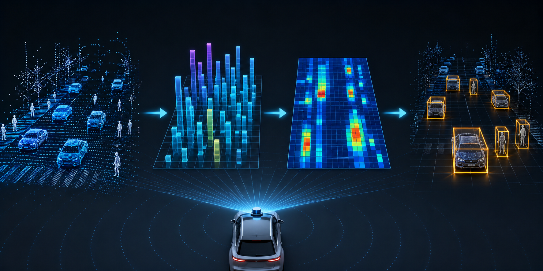
上一篇我们学习了PointNet,理解了如何用深度学习直接处理无序点云。但PointNet主要用于分类和分割,离"实时检测周围的车辆"还有距离。这一篇我们来看PointPillars------一个能让自动驾驶汽车以62 FPS实时检测3D目标的网络,真正能让工业使用的网络。
一、从PointNet到3D目标检测(先搞清楚问题)
1.1 PointNet解决了什么?
PointNet的贡献:
✅ 直接处理无序点云
✅ 学习全局特征
✅ 端到端训练

PointNet没解决的:
❌ 只有全局特征,缺乏局部特征
❌ 无法定位物体在3D空间中的位置
❌ 不能做实时推理(太慢)
1.2 3D目标检测要做什么?
输入:一堆3D点(激光雷达扫描)
输出:每个物体的3D边界框

具体来说:
┌─────────────────────────────────────────┐
│  输出:                                  │
│  - 物体类别(车、行人、自行车)          │
│  - 3D位置 (x, y, z)                     │
│  - 3D尺寸 (长, 宽, 高)                  │
│  - 朝向角 (yaw)                         │
│  - 置信度                               │
└─────────────────────────────────────────┘直观理解:
激光雷达扫描一圈:

        *  *  *
      *  *  *  *  *          ← 车的点云
    *  *  *  *  *  *  *

                          *  *  *  ← 行人的点云
                        *  *  *
                          *

网络要做的:
1. 哪些点属于车?→ 画一个3D框
2. 哪些点属于行人?→ 画另一个3D框
3. 每个框的位置、大小、朝向是什么?
1.3 为什么不能直接用PointNet做检测?
PointNet的问题:

1. 全局特征 → 只知道"这是什么",不知道"在哪里"
   - max pooling把所有点的信息压缩成一个向量
   - 丢失了空间位置信息

2. 没有局部特征 → 无法区分不同物体
   - 车和行人的点混在一起
   - PointNet会把它们混为一谈

3. 计算量大 → 无法实时
   - 自动驾驶需要 ≥30 FPS
   - PointNet处理一帧要几百毫秒
1.4 3D检测的发展路线
PointNet (2017)
    │  直接处理点云,但只能分类/分割
    ↓
PointNet++ (2017)
    │  加入局部特征,层次化学习
    ↓
VoxelNet (2018)
    │  把点云转成体素,用3D卷积
    │  效果好,但太慢(~2 FPS)
    ↓
SECOND (2018)
    │  用稀疏卷积加速VoxelNet
    │  速度提升,但还是不够快
    ↓
PointPillars (2019)
    │  用"柱子"代替体素,2D卷积处理
    │  62 FPS!实时!
    ↓
    自动驾驶实际部署
二、PointPillars的核心思想(最重要的部分)
2.1 一句话概括
把3D点云按柱子(Pillar)分组,编码成2D伪图像,然后用成熟的2D检测网络做目标检测。
2.2 为什么叫"PointPillars"?
Pillar = 柱子

把3D空间沿Z轴切成一根根"柱子":

俯视图(XY平面):
┌───┬───┬───┬───┬───┐
│   │ P │   │ P │   │    P = Pillar(柱子)
├───┼───┼───┼───┼───┤
│ P │ P │ P │   │ P │    每个柱子沿Z轴延伸
├───┼───┼───┼───┼───┤    柱子内的所有点归为一组
│   │   │ P │ P │   │
├───┼───┼───┼───┼───┤
│   │ P │   │   │ P │
└───┴───┴───┴───┴───┘

侧视图(XZ平面):
        ┃     ┃
        ┃     ┃           ← 柱子沿Z轴延伸
        ┃     ┃
    ━━━━┻━━━━━┻━━━━       ← 地面
2.3 PointPillars的三大步骤
步骤1:点云 → 柱子(Pillarization)
  把点云按照XY平面划分成网格,每个格子是一根柱子

步骤2:柱子 → 伪图像(Pseudo Image)
  对每根柱子内的点提取特征,编码成一个2D特征图

步骤3:伪图像 → 3D检测框(Detection)
用2D卷积网络(类似YOLO)检测,输出3D边界框图解整体流程:
输入点云 [N×4]
(N个点,每个点有x,y,z,intensity)
        │
        ↓
┌─────────────────────────────────────┐
│ 步骤1:柱子化(Pillarization)       │
│                                     │
│ - XY平面划分网格(如0.16m×0.16m)   │
│ - 每个网格是一根柱子                 │
│ - 点按XY坐标分配到对应柱子          │
└─────────────────────────────────────┘
        │
        ↓
┌─────────────────────────────────────┐
│ 步骤2:柱子特征编码(Pillar Encoder)│
│                                     │
│ - 每根柱子内的点用简化PointNet处理  │
│ - 提取柱子级特征                    │
│ - 映射到2D网格 → 伪图像            │
└─────────────────────────────────────┘
        │
        ↓
   伪图像 [C×H×W]
   (通道×高度×宽度)
        │
        ↓
┌─────────────────────────────────────┐
│ 步骤3:2D检测网络(Detection Head)  │
│                                     │
│ - 类似YOLO的2D卷积骨干网络          │
│ - 特征金字塔(FPN)多尺度检测       │
│ - 输出:类别 + 2D框 + 高度 + 朝向   │
└─────────────────────────────────────┘
        │
        ↓
3D检测结果:
  - 类别:车辆/行人/自行车
  - 位置:(x, y, z)
  - 尺寸:(长, 宽, 高)
  - 朝向:yaw角
2.4 为什么这样做很快?
对比其他方法:

VoxelNet:
  3D体素 → 3D卷积 → 检测
  问题:3D卷积计算量巨大

SECOND:
  3D体素 → 稀疏3D卷积 → 检测
  改进:稀疏卷积减少计算
  问题:实现复杂,仍有3D卷积

PointPillars:
  柱子 → 2D特征图 → 2D卷积 → 检测
  优势:完全避免3D卷积!
        2D卷积有高度优化的实现(cuDNN)
        可以直接用成熟的2D检测框架

速度对比:
┌──────────────┬──────────┬──────────┐
│ 方法         │ FPS      │ 3D卷积? │
├──────────────┼──────────┼──────────┤
│ VoxelNet     │ ~2       │ 是       │
│ SECOND       │ ~20      │ 稀疏     │
│ PointPillars │ ~62      │ 否!     │
└──────────────┴──────────┴──────────┘
三、PointPillars的网络结构详解
3.1 步骤1:柱子化(Pillarization)
核心操作:把点云按XY坐标分配到网格中
python
def pillarize(point_cloud, x_range, y_range, pillar_size):
    """
    将点云分配到柱子中

    参数:
        point_cloud: [N, 4] - N个点,每个点(x,y,z,intensity)
        x_range: (x_min, x_max) - X方向范围
        y_range: (y_min, y_max) - Y方向范围
        pillar_size: (dx, dy) - 每个柱子的XY尺寸

    返回:
        pillars: 每个柱子内的点列表
    """
    x_min, x_max = x_range
    y_min, y_max = y_range
    dx, dy = pillar_size

    # 计算网格数量
    x_bins = int((x_max - x_min) / dx)  # 例如 432
    y_bins = int((y_max - y_min) / dy)  # 例如 496

    # 计算每个点属于哪个柱子
    x_idx = ((point_cloud[:, 0] - x_min) / dx).astype(int)
    y_idx = ((point_cloud[:, 1] - y_min) / dy).astype(int)

    # 过滤超出范围的点
    valid = (x_idx >= 0) & (x_idx < x_bins) & \
            (y_idx >= 0) & (y_idx < y_bins)

    # 按柱子分组
    pillars = {}
    for i in range(len(point_cloud)):
        if valid[i]:
            key = (x_idx[i], y_idx[i])
            if key not in pillars:
                pillars[key] = []
            pillars[key].append(point_cloud[i])

return pillars, (x_bins, y_bins)图解:
原始点云:                  柱子化后:
    *  *                        ┌───┬───┬───┐
  *      *                      │P0 │P1 │   │
 *   *    *          →          ├───┼───┼───┤
  *      *                      │P2 │P3 │P4 │
    *  *                        ├───┼───┼───┤
                                │   │P5 │   │
                                └───┴───┴───┘

P0 = [点A, 点B]     ← 柱子0内的所有点
P1 = [点C, 点D, 点E]
...
3.2 步骤2:柱子特征编码(Pillar Encoder)
核心思想:对每根柱子内的点,用简化版PointNet提取特征
python
class PillarEncoder(nn.Module):
    """柱子特征编码器"""

    def __init__(self, in_channels=4, out_channels=64):
        """
        in_channels: 输入通道数(x,y,z,intensity)
        out_channels: 输出特征通道数
        """
        super().__init__()

        # 简化的PointNet:对每个点提取特征
        self.point_net = nn.Sequential(
            nn.Linear(in_channels + 7, 64),  # +7是因为要拼接额外特征
            nn.BatchNorm1d(64),
            nn.ReLU(),
            nn.Linear(64, 64),
            nn.BatchNorm1d(64),
            nn.ReLU(),
        )

    def forward(self, pillars, indices, num_points):
        """
        pillars: [M, max_points, 4] - M根柱子,每根最多max_points个点
        indices: [M, 2] - 每根柱子在网格中的(x,y)索引
        num_points: [M] - 每根柱子实际有多少个点

        返回:
        pseudo_image: [C, H, W] - 伪图像
        """
        M, max_points, C = pillars.shape

        # 1. 计算额外特征
        # 每个点相对于柱子中心的偏移
        center = pillars[:, :, :3].mean(dim=1, keepdim=True)  # [M, 1, 3]
        offset = pillars[:, :, :3] - center  # [M, max_points, 3]

        # 每个点相对于柱子中心的XY偏移
        pillar_center_xy = torch.zeros_like(pillars[:, :, :2])
        pillar_center_xy[:, :, 0] = indices[:, 0].unsqueeze(1)  # x索引
        pillar_center_xy[:, :, 1] = indices[:, 1].unsqueeze(1)  # y索引

        # 拼接所有特征
        features = torch.cat([
            pillars,           # [M, max_points, 4] 原始坐标+强度
            offset,            # [M, max_points, 3] 相对偏移
            pillar_center_xy,  # [M, max_points, 2] 柱子中心
        ], dim=-1)  # [M, max_points, 4+3+2=9]

        # 2. 用PointNet提取特征
        features = features.view(M * max_points, -1)
        features = self.point_net(features)  # [M*max_points, 64]
        features = features.view(M, max_points, -1)

        # 3. 最大值池化(聚合柱子内所有点)
        # 用num_points创建mask
        mask = torch.arange(max_points).unsqueeze(0) < num_points.unsqueeze(1)
        mask = mask.unsqueeze(-1).float()  # [M, max_points, 1]

        features = features * mask  # 屏蔽无效点
        pillar_feature = torch.max(features, dim=1)[0]  # [M, 64]

        return pillar_feature
关键细节:拼接额外特征
原始特征:(x, y, z, intensity) → 4维
额外特征:
  - 相对于柱子中心的偏移 (Δx, Δy, Δz) → 3维
  - 柱子中心的网格坐标 → 2维

总计:4 + 3 + 2 = 9维

为什么要这样做?
1. 偏移量 → 告诉网络点在柱子内的相对位置
2. 网格坐标 → 告诉网络这个柱子在全局的位置
3. 这样最大值池化后不会丢失位置信息
3.3 步骤3:生成伪图像
python
def create_pseudo_image(pillar_features, indices, grid_size):
    """
    将柱子特征映射到2D网格,生成伪图像

    参数:
        pillar_features: [M, 64] - M根柱子的特征
        indices: [M, 2] - 每根柱子的网格索引
        grid_size: (H, W) - 网格大小

    返回:
        pseudo_image: [64, H, W] - 伪图像
    """
    C = pillar_features.shape[1]
    H, W = grid_size

    # 创建空白图像
    pseudo_image = torch.zeros(C, H, W)

    # 将柱子特征填入对应位置
    for i in range(len(pillar_features)):
        x, y = indices[i]
        pseudo_image[:, y, x] = pillar_features[i]

return pseudo_image图解:
柱子特征:
  柱子(0,0) → 特征向量 f0
  柱子(1,0) → 特征向量 f1
  柱子(2,1) → 特征向量 f2
  ...

映射到2D网格:
┌───┬───┬───┬───┬───┐
│f0 │f1 │ 0 │ 0 │ 0 │    0 = 空柱子(没有点)
├───┼───┼───┼───┼───┤
│ 0 │ 0 │f2 │ 0 │ 0 │    每个格子是一个64维向量
├───┼───┼───┼───┼───┤
│ 0 │ 0 │ 0 │f3 │ 0 │
└───┴───┴───┴───┴───┘

这就是"伪图像"!
看起来像图像,但每个"像素"是64维特征
可以直接用2D卷积处理
3.4 步骤4:2D检测网络(Backbone + Detection Head)
python
class PointPillarsBackbone(nn.Module):
    """PointPillars的2D骨干网络"""

    def __init__(self, in_channels=64):
        super().__init__()

        # Block 1:下采样
        self.block1 = nn.Sequential(
            nn.Conv2d(in_channels, 64, 3, stride=2, padding=1),
            nn.BatchNorm2d(64),
            nn.ReLU(),
            nn.Conv2d(64, 64, 3, stride=1, padding=1),
            nn.BatchNorm2d(64),
            nn.ReLU(),
            nn.Conv2d(64, 64, 3, stride=1, padding=1),
            nn.BatchNorm2d(64),
            nn.ReLU(),
        )

        # Block 2:继续下采样
        self.block2 = nn.Sequential(
            nn.Conv2d(64, 128, 3, stride=2, padding=1),
            nn.BatchNorm2d(128),
            nn.ReLU(),
            nn.Conv2d(128, 128, 3, stride=1, padding=1),
            nn.BatchNorm2d(128),
            nn.ReLU(),
            nn.Conv2d(128, 128, 3, stride=1, padding=1),
            nn.BatchNorm2d(128),
            nn.ReLU(),
        )

        # Block 3:最深层
        self.block3 = nn.Sequential(
            nn.Conv2d(128, 256, 3, stride=2, padding=1),
            nn.BatchNorm2d(256),
            nn.ReLU(),
            nn.Conv2d(256, 256, 3, stride=1, padding=1),
            nn.BatchNorm2d(256),
            nn.ReLU(),
            nn.Conv2d(256, 256, 3, stride=1, padding=1),
            nn.BatchNorm2d(256),
            nn.ReLU(),
        )

    def forward(self, x):
        """
        x: [B, 64, H, W] - 伪图像
        返回:多尺度特征列表
        """
        x1 = self.block1(x)   # [B, 64, H/2, W/2]
        x2 = self.block2(x1)  # [B, 128, H/4, W/4]
        x3 = self.block3(x2)  # [B, 256, H/8, W/8]

return [x1, x2, x3]特征金字塔网络(FPN):
python
class FPN(nn.Module):
    """特征金字塔网络,融合多尺度特征"""

    def __init__(self):
        super().__init__()

        # 横向连接(将通道数统一)
        self.lateral1 = nn.Conv2d(64, 128, 1)
        self.lateral2 = nn.Conv2d(128, 128, 1)
        self.lateral3 = nn.Conv2d(256, 128, 1)

        # 输出平滑
        self.smooth = nn.Sequential(
            nn.Conv2d(128, 128, 3, padding=1),
            nn.BatchNorm2d(128),
            nn.ReLU(),
        )

    def forward(self, features):
        """
        features: [x1, x2, x3] 多尺度特征
        返回:融合后的特征图
        """
        x1, x2, x3 = features

        # 从深层到浅层融合
        p3 = self.lateral3(x3)  # [B, 128, H/8, W/8]

        p2 = self.lateral2(x2) + \
             nn.functional.interpolate(p3, scale_factor=2)  # [B, 128, H/4, W/4]

        p1 = self.lateral1(x1) + \
             nn.functional.interpolate(p2, scale_factor=2)  # [B, 128, H/2, W/2]

        # 平滑
        out = self.smooth(p1)  # [B, 128, H/2, W/2]

return out检测头:
python
class DetectionHead(nn.Module):
    """检测头,预测类别和边界框"""

    def __init__(self, in_channels=128, num_classes=3, num_anchors=2):
        """
        num_classes: 类别数(车、行人、自行车)
        num_anchors: 每个位置的锚框数量
        """
        super().__init__()
        self.num_classes = num_classes
        self.num_anchors = num_anchors

        # 分类头:预测每个锚框的类别
        self.cls_head = nn.Conv2d(
            in_channels, num_anchors * num_classes, 1
        )

        # 回归头:预测边界框参数
        # 每个框有7个参数:(x, y, z, w, l, h, yaw)
        self.reg_head = nn.Conv2d(
            in_channels, num_anchors * 7, 1
        )

        # 方向头:预测朝向(正面/背面)
        self.dir_head = nn.Conv2d(
            in_channels, num_anchors * 2, 1
        )

    def forward(self, x):
        """
        x: [B, 128, H, W] - FPN输出的特征图
        返回:
            cls: [B, H*W*num_anchors, num_classes] - 分类得分
            reg: [B, H*W*num_anchors, 7] - 边界框参数
            dir: [B, H*W*num_anchors, 2] - 朝向分类
        """
        B, C, H, W = x.shape

        # 分类预测
        cls = self.cls_head(x)  # [B, num_anchors*num_classes, H, W]
        cls = cls.permute(0, 2, 3, 1)  # [B, H, W, num_anchors*num_classes]
        cls = cls.reshape(B, -1, self.num_classes)

        # 回归预测
        reg = self.reg_head(x)  # [B, num_anchors*7, H, W]
        reg = reg.permute(0, 2, 3, 1)  # [B, H, W, num_anchors*7]
        reg = reg.reshape(B, -1, 7)

        # 方向预测
        dir = self.dir_head(x)  # [B, num_anchors*2, H, W]
        dir = dir.permute(0, 2, 3, 1)  # [B, H, W, num_anchors*2]
        dir = dir.reshape(B, -1, 2)

        return cls, reg, dir
四、完整的PointPillars代码
4.1 完整网络
python
import torch
import torch.nn as nn

class PointPillars(nn.Module):
    """完整的PointPillars网络"""

    def __init__(self, num_classes=3):
        """
        num_classes: 检测类别数
        默认3:车辆、行人、自行车
        """
        super().__init__()

        # 1. 柱子编码器
        self.pillar_encoder = PillarEncoder(
            in_channels=4,   # x, y, z, intensity
            out_channels=64
        )

        # 2. 2D骨干网络
        self.backbone = PointPillarsBackbone(in_channels=64)

        # 3. 特征金字塔
        self.fpn = FPN()

        # 4. 检测头
        self.detection_head = DetectionHead(
            in_channels=128,
            num_classes=num_classes,
            num_anchors=2
        )

    def forward(self, pillars, indices, num_points, grid_size):
        """
        pillars: [M, max_points, 4] - 柱子内的点
        indices: [M, 2] - 柱子的网格索引
        num_points: [M] - 每根柱子的点数
        grid_size: (H, W) - 网格大小

        返回:
        cls: 分类得分
        reg: 边界框参数
        dir: 朝向分类
        """
        # 1. 编码柱子特征
        pillar_features = self.pillar_encoder(
            pillars, indices, num_points
        )  # [M, 64]

        # 2. 生成伪图像
        pseudo_image = create_pseudo_image(
            pillar_features, indices, grid_size
        )  # [64, H, W]
        pseudo_image = pseudo_image.unsqueeze(0)  # [1, 64, H, W]

        # 3. 2D骨干网络
        features = self.backbone(pseudo_image)

        # 4. 特征金字塔融合
        fused = self.fpn(features)  # [1, 128, H/2, W/2]

        # 5. 检测
        cls, reg, dir = self.detection_head(fused)

        return cls, reg, dir
4.2 锚框设计
python
class AnchorGenerator:
    """锚框生成器"""

    def __init__(self):
        # 不同类别的锚框尺寸
        # 格式:(长, 宽, 高)
        self.anchors = {
            'vehicle': (4.0, 1.6, 1.5),      # 车辆
            'pedestrian': (0.8, 0.6, 1.7),   # 行人
            'cyclist': (1.8, 0.6, 1.7),       # 自行车
        }

    def generate(self, grid_size, anchor_sizes):
        """
        为每个网格位置生成锚框

        参数:
            grid_size: (H, W) - 网格大小
            anchor_sizes: 锚框尺寸列表

        返回:
            anchors: [H*W*num_anchors, 7] - 锚框
            格式:(x, y, z, w, l, h, yaw)
        """
        H, W = grid_size
        anchors = []

        for i in range(H):
            for j in range(W):
                # 网格中心坐标
                x = j * pillar_size + pillar_size / 2
                y = i * pillar_size + pillar_size / 2

                for size in anchor_sizes:
                    l, w, h = size
                    z = h / 2  # 锚框底部在地面

                    # 两个朝向:0度和90度
                    for yaw in [0, 1.57]:  # 0和π/2
                        anchors.append([x, y, z, w, l, h, yaw])

        return torch.FloatTensor(anchors)
4.3 损失函数
python
class PointPillarsLoss(nn.Module):
    """PointPillars的损失函数"""

    def __init__(self):
        super().__init__()

        # 分类损失
        self.cls_loss = nn.FocalLoss(alpha=0.25, gamma=2)

        # 回归损失(Smooth L1)
        self.reg_loss = nn.SmoothL1Loss(reduction='none')

        # 方向损失
        self.dir_loss = nn.CrossEntropyLoss(reduction='none')

    def forward(self, pred_cls, pred_reg, pred_dir,
                target_cls, target_reg, target_dir, mask):
        """
        pred_cls: [B, N, num_classes] - 预测分类
        pred_reg: [B, N, 7] - 预测回归
        pred_dir: [B, N, 2] - 预测方向
        target_cls: [B, N] - 目标分类
        target_reg: [B, N, 7] - 目标回归
        target_dir: [B, N] - 目标方向
        mask: [B, N] - 正样本mask
        """
        # 1. 分类损失(所有样本)
        cls_loss = self.cls_loss(pred_cls, target_cls)

        # 2. 回归损失(仅正样本)
        reg_loss = self.reg_loss(pred_reg, target_reg)
        reg_loss = reg_loss * mask.unsqueeze(-1)
        reg_loss = reg_loss.sum() / (mask.sum() + 1e-6)

        # 3. 方向损失(仅正样本)
        dir_loss = self.dir_loss(pred_dir, target_dir)
        dir_loss = dir_loss * mask
        dir_loss = dir_loss.sum() / (mask.sum() + 1e-6)

        # 总损失
        total_loss = cls_loss + 2 * reg_loss + 0.2 * dir_loss

        return total_loss, cls_loss, reg_loss, dir_loss
4.4 训练代码
python
def train_pointpillars():
    # 1. 创建模型
    model = PointPillars(num_classes=3)
    model = model.cuda()

    # 2. 优化器
    optimizer = torch.optim.Adam(
        model.parameters(), lr=0.001, weight_decay=0.01
    )
    scheduler = torch.optim.lr_scheduler.CosineAnnealingLR(
        optimizer, T_max=160
    )

    # 3. 损失函数
    criterion = PointPillarsLoss()

    # 4. 训练循环
    for epoch in range(160):
        model.train()
        total_loss = 0

        for batch in train_loader:
            # 解包数据
            pillars = batch['pillars'].cuda()
            indices = batch['indices'].cuda()
            num_points = batch['num_points'].cuda()
            targets = batch['targets']

            # 前向传播
            pred_cls, pred_reg, pred_dir = model(
                pillars, indices, num_points, grid_size
            )

            # 计算损失
            loss, cls_loss, reg_loss, dir_loss = criterion(
                pred_cls, pred_reg, pred_dir,
                targets['cls'].cuda(),
                targets['reg'].cuda(),
                targets['dir'].cuda(),
                targets['mask'].cuda()
            )

            # 反向传播
            optimizer.zero_grad()
            loss.backward()
            optimizer.step()

            total_loss += loss.item()

        # 更新学习率
        scheduler.step()

        # 打印统计
        print(f'Epoch {epoch+1}, Loss: {total_loss/len(train_loader):.4f}')

        # 验证
        if (epoch + 1) % 10 == 0:
            evaluate(model, val_loader)
五、PointPillars vs 其他方法(效果对比)
5.1 KITTI数据集上的性能对比
KITTI 3D检测基准(汽车类别,Moderate难度):

┌─────────────────┬───────────┬───────────┬───────────┐
│ 方法            │ AP Easy   │ AP Mod    │ AP Hard   │
├─────────────────┼───────────┼───────────┼───────────┤
│ VoxelNet        │ 81.97     │ 65.46     │ 62.85     │
│ SECOND          │ 83.13     │ 68.20     │ 64.57     │
│ PointPillars    │ 82.58     │ 74.31     │ 68.99     │
└─────────────────┴───────────┴───────────┴───────────┘

速度对比:
┌─────────────────┬───────────┬──────────────┐
│ 方法            │ FPS       │ 推理时间     │
├─────────────────┼───────────┼──────────────┤
│ VoxelNet        │ ~2        │ ~500ms       │
│ SECOND          │ ~20       │ ~50ms        │
│ PointPillars    │ ~62       │ ~16ms        │
└─────────────────┴───────────┴──────────────┘
5.2 为什么PointPillars既快又准?
1. 避免3D卷积
   - 3D卷积计算量 O(N³)
   - 2D卷积计算量 O(N²)
   - 差一个数量级!

2. 柱子设计的巧妙之处
   - 体素:3D网格,大部分是空的 → 浪费计算
   - 柱子:只在XY平面划分,Z轴不分 → 自然稀疏

3. 利用成熟的2D检测框架
   - FPN、锚框、NMS都是2D检测的成熟技术
   - 不需要重新发明轮子

4. 工程优化
   - 2D卷积有cuDNN高度优化
   - 可以直接用TensorRT加速
5.3 PointPillars的局限性
1. 柱子化会丢失Z轴细节
   - 高度信息被压缩成特征
   - 对于高度差异大的物体(如立着的人 vs 躺着的人)可能不敏感

2. 固定的柱子大小
   - 小物体可能在一个柱子里信息不足
   - 大物体可能跨多个柱子,需要后处理

3. 锚框设计需要先验知识
   - 不同数据集需要不同的锚框尺寸
   - 需要根据数据统计设计
六、PointPillars在自动驾驶中的实际应用
6.1 传感器配置
典型的自动驾驶传感器配置:

        ┌──── 激光雷达(顶部)────┐
        │     360° 扫描           │
        │     64线/128线          │
        └─────────────────────────┘
                  │
    ┌─────────────┼─────────────┐
    │             │             │
  前摄像头     左/右摄像头    后摄像头
    │             │             │
    └─────────────┼─────────────┘
                  │
        ┌─────────┴─────────┐
        │   PointPillars    │
        │   处理激光雷达    │
        │   输出3D检测框    │
        └───────────────────┘
6.2 完整的检测流水线
python
class AutonomousDrivingPipeline:
    """自动驾驶3D检测流水线"""

    def __init__(self):
        self.model = PointPillars(num_classes=3)
        self.model.load_state_dict(torch.load('checkpoint.pth'))
        self.model.eval()

        # 后处理参数
        self.nms_threshold = 0.5
        self.score_threshold = 0.3

    def detect(self, point_cloud):
        """
        输入:原始点云 [N, 4]
        输出:检测结果列表
        """
        # 1. 预处理
        pillars, indices, num_points = self.preprocess(point_cloud)

        # 2. 模型推理
        with torch.no_grad():
            cls, reg, dir = self.model(
                pillars, indices, num_points, grid_size
            )

        # 3. 后处理
        boxes = self.postprocess(cls, reg, dir)

        return boxes

    def preprocess(self, point_cloud):
        """点云预处理"""
        # 过滤地面点
        point_cloud = point_cloud[point_cloud[:, 2] > -1.5]

        # 过滤远处的点
        point_cloud = point_cloud[
            (point_cloud[:, 0] > 0) & (point_cloud[:, 0] < 70) &
            (point_cloud[:, 1] > -40) & (point_cloud[:, 1] < 40)
        ]

        # 柱子化
        pillars, grid = pillarize(
            point_cloud,
            x_range=(0, 70),
            y_range=(-40, 40),
            pillar_size=(0.16, 0.16)
        )

        return pillars, grid

    def postprocess(self, cls, reg, dir):
        """后处理:解码、NMS"""
        # 解码边界框
        boxes = self.decode_boxes(reg)

        # 过滤低置信度
        scores = torch.softmax(cls, dim=-1).max(dim=-1)[0]
        mask = scores > self.score_threshold
        boxes = boxes[mask]
        scores = scores[mask]

        # NMS
        keep = self.nms(boxes, scores, self.nms_threshold)
        boxes = boxes[keep]

        return boxes
6.3 实际部署考虑
1. 模型优化
   - 使用TensorRT加速
   - FP16推理(半精度浮点)
   - 量化(INT8)

2. 工程优化
   - 点云预处理用CUDA加速
   - 柱子化用自定义CUDA kernel
   - NMS用GPU实现

3. 实际性能
   - 原始PointPillars:62 FPS
   - TensorRT优化后:100+ FPS
   - INT8量化后:200+ FPS
七、PointPillars vs 其他3D检测方法
7.1 方法对比
按数据表示分类:

1. 基于体素的方法
   VoxelNet → SECOND → ...
   - 优点:保留3D结构
   - 缺点:计算量大

2. 基于点的方法
   PointNet → PointNet++ → ...
   - 优点:保留原始点
   - 缺点:密度不均匀时不稳定

3. 基于柱子的方法
   PointPillars
   - 优点:速度快,部署简单
   - 缺点:Z轴信息压缩

4. 基于BEV(鸟瞰图)的方法
   BEVDet → BEVFormer → ...
   - 优点:多传感器融合方便
   - 缺点:需要相机-LiDAR标定
7.2 如何选择?
选择PointPillars的场景:
✅ 需要实时推理(>30 FPS)
✅ 只有激光雷达输入
✅ 嵌入式部署(算力有限)
✅ 快速原型开发

选择其他方法的场景:
- 需要更高精度 → SECOND, CenterPoint
- 需要多传感器融合 → BEVFormer, TransFusion
- 需要处理稀疏点云 → 3D-SSD, SA-SSD
八、常见问题解答(FAQ)
Q1: PointPillars为什么比VoxelNet快那么多?
答:
核心原因:避免了3D卷积

VoxelNet:
  3D体素 → 3D卷积 → 3D特征 → 检测
  3D卷积计算量:O(C × D × H × W × k³)
  其中k是卷积核大小(通常为3)

PointPillars:
  柱子 → 2D伪图像 → 2D卷积 → 检测
  2D卷积计算量:O(C × H × W × k²)

差一个数量级!
而且2D卷积有cuDNN高度优化
Q2: 柱子大小怎么选?
答:
柱子大小影响精度和速度:

小柱子(0.1m × 0.1m):
  - 精度高(保留更多细节)
  - 伪图像大(计算量大)
  - 速度慢

大柱子(0.2m × 0.2m):
  - 精度低(细节丢失)
  - 伪图像小(计算量小)
  - 速度快

常用设置:
  KITTI数据集:0.16m × 0.16m
  nuScenes数据集:0.2m × 0.2m
Q3: 每根柱子最多保留多少个点?
答:
通常设置:max_points = 32 或 64

原因:
- 大部分柱子只有几个点
- 设置上限避免内存爆炸
- 超过上限的点随机采样

实验表明:
- max_points = 32 足够
- 增加到64精度提升很小
- 但内存和计算量增加
Q4: PointPillars能检测多远的物体?
答:
取决于激光雷达和设置:

典型设置:
- X方向:0m ~ 70m
- Y方向:-40m ~ 40m
- Z方向:-3m ~ 1m

远处物体的问题:
- 点数少(稀疏)
- 特征不足
- 检测困难

改进方法:
- 多尺度检测
- 远处用更大的柱子
- 结合相机图像
Q5: PointPillars还能怎么改进?
答:
1. 加入注意力机制
   - Pillar Attention
   - 自适应特征聚合

2. 多传感器融合
   - 相机 + LiDAR
   - 融合图像特征

3. 时序信息
   - 融合多帧点云
   - 速度估计

4. 更好的骨干网络
   - ResNet, EfficientNet
   - 用更大的网络提升精度

5. 无锚框方法
   - CenterPoint
   - 去掉锚框设计
九、从PointPillars到3D占用感知
9.1 PointPillars的输出是什么?
PointPillars输出:
- 3D边界框列表
- 每个框:位置 + 尺寸 + 朝向 + 类别

问题:
- 只能检测已知类别
- 无法处理不规则物体
- 对遮挡敏感
9.2 3D占用感知的优势
3D占用感知输出:
- 3D体素网格
- 每个体素:占用/空 + 类别

优势:
- 可以表示任意形状
- 对遮挡更鲁棒
- 可以处理未知物体

从PointPillars到占用感知:
PointPillars:点云 → 柱子 → 伪图像 → 检测框
占用感知:  点云/图像 → 特征 → 3D占用网格
9.3 知识迁移
PointPillars学到的知识:
1. 柱子化 → 高效的点云表示
2. 2D卷积 → 避免3D卷积的计算量
3. 特征金字塔 → 多尺度特征融合
4. 锚框设计 → 目标检测的先验知识

这些知识可以直接迁移到占用感知:
- 柱子化 → 体素化
- 2D卷积 → 3D稀疏卷积
- 特征金字塔 → 3D特征金字塔
- 检测头 → 分割头
十、总结:PointPillars的精髓
10.1 核心思想
- 柱子化:把3D点云按XY平面分组,避免3D卷积
- 伪图像:将柱子特征映射到2D网格,利用成熟的2D检测
- 端到端:从原始点云到3D检测框,完全可训练
- 实时性:62 FPS,满足自动驾驶实时要求
10.2 一句话总结
PointPillars通过将点云组织成柱子并编码为伪图像,巧妙地将3D检测转化为2D检测,实现了速度和精度的完美平衡。
10.3 关键创新
| 创新 | 作用 |
|---|---|
| 柱子化 | 避免3D卷积,高效表示 |
| 伪图像 | 利用2D检测成熟技术 |
| 简化PointNet | 柱子内特征提取 |
| 特征金字塔 | 多尺度特征融合 |
10.4 下一步学习
- CenterPoint:无锚框的3D检测
- BEVFormer:鸟瞰图视角的多传感器融合
- 3D占用感知:从检测到分割
附录:关键术语表
| 术语 | 英文 | 含义 |
|---|---|---|
| 柱子 | Pillar | XY平面上的一个网格单元 |
| 伪图像 | Pseudo Image | 柱子特征映射成的2D特征图 |
| 锚框 | Anchor | 预定义的参考边界框 |
| NMS | Non-Maximum Suppression | 非极大值抑制,去除重复检测 |
| FPN | Feature Pyramid Network | 特征金字塔网络 |
| FPS | Frames Per Second | 每秒处理帧数 |
| BEV | Bird's Eye View | 鸟瞰图视角 |
| 激光雷达 | LiDAR | 光探测和测距传感器 |
| 体素 | Voxel | 3D像素,体积元素 |
下期预告:《从检测到感知------3D占用网格如何让自动驾驶"看穿"遮挡?》