Ultralytics:解读SPPF模块
- 前言
- 相关介绍
-
- [Ultralytics 简介](#Ultralytics 简介)
- 前提条件
- 实验环境
- [SPPF(空间金字塔池化 - 快速版)](#SPPF(空间金字塔池化 - 快速版))
- 参考文献
前言
- 由于本人水平有限,难免出现错漏,敬请批评改正。
- 更多精彩内容,可点击进入Python日常小操作专栏、OpenCV-Python小应用专栏、YOLO系列专栏、自然语言处理专栏、人工智能混合编程实践专栏或我的个人主页查看
- YOLOs-CPP:一个免费开源的YOLO全系列C++推理库(以YOLO26为例)
- PaddleOCR:Win10上安装使用PPOCRLabel标注工具
- 目标检测:使用自己的数据集微调DEIMv2进行物体检测
- 图像分割:PyTorch从零开始实现SegFormer语义分割
- 图像超分:使用自己的数据集微调Real-ESRGAN-x4plus进行超分重建
- 图像生成:PyTorch从零开始实现一个简单的扩散模型
- Stable Diffusion:使用自己的数据集微调 Stable Diffusion 3.5 LoRA 文生图模型
- 图像超分:使用自己的数据集微调Real-ESRGAN-x2plus进行超分重建
- Anomalib:使用Anomalib 2.1.0训练自己的数据集进行异常检测
- Anomalib:在Linux服务器上安装使用Anomalib 2.1.0
- 人工智能混合编程实践:C++调用封装好的DLL进行异常检测推理
- 人工智能混合编程实践:C++调用封装好的DLL进行FP16图像超分重建(v3.0)
- 隔离系统Python:源码编译3.11.8到自定义目录(含PGO性能优化)
- 在线机的Python环境迁移到离线机上
- Nuitka 将 Python 脚本封装为 .pyd 或 .so 文件
- Ultralytics:使用 YOLO11 进行速度估计
- Ultralytics:使用 YOLO11 进行物体追踪
- Ultralytics:使用 YOLO11 进行物体计数
- Ultralytics:使用 YOLO11 进行目标打码
- 人工智能混合编程实践:C++调用Python ONNX进行YOLOv8推理
- 人工智能混合编程实践:C++调用封装好的DLL进行YOLOv8实例分割
- 人工智能混合编程实践:C++调用Python ONNX进行图像超分重建
- 人工智能混合编程实践:C++调用Python AgentOCR进行文本识别
- 通过计算实例简单地理解PatchCore异常检测
- Python将YOLO格式实例分割数据集转换为COCO格式实例分割数据集
- YOLOv8 Ultralytics:使用Ultralytics框架训练RT-DETR实时目标检测模型
- 基于DETR的人脸伪装检测
- YOLOv7训练自己的数据集(口罩检测)
- YOLOv8训练自己的数据集(足球检测)
- YOLOv5:TensorRT加速YOLOv5模型推理
- YOLOv5:IoU、GIoU、DIoU、CIoU、EIoU
- 玩转Jetson Nano(五):TensorRT加速YOLOv5目标检测
- YOLOv5:添加SE、CBAM、CoordAtt、ECA注意力机制
- YOLOv5:yolov5s.yaml配置文件解读、增加小目标检测层
- Python将COCO格式实例分割数据集转换为YOLO格式实例分割数据集
- YOLOv5:使用7.0版本训练自己的实例分割模型(车辆、行人、路标、车道线等实例分割)
- 使用Kaggle GPU资源免费体验Stable Diffusion开源项目
- Stable Diffusion:在服务器上部署使用Stable Diffusion WebUI进行AI绘图(v2.0)
- Stable Diffusion:使用自己的数据集微调训练LoRA模型(v2.0)
相关介绍
Ultralytics 简介
Ultralytics 基于多年的计算机视觉和人工智能基础研究,创建了最先进的 (SOTA) YOLO 模型。我们的模型不断更新性能和灵活性,快速、准确且易于使用。他们擅长对象检测、跟踪、实例分割、语义分割、图像分类和姿势估计任务。
前提条件
- 熟悉Python、Pytorch
实验环境
bash
Package                  Version
------------------------ ------------
Python                   3.11.8
absl-py                  2.4.0
accelerate               1.13.0
annotated-doc            0.0.4
anyio                    4.13.0
calflops                 0.3.2
certifi                  2026.4.22
charset-normalizer       3.4.7
click                    8.3.3
colorama                 0.4.6
contourpy                1.3.3
cycler                   0.12.1
filelock                 3.29.0
flatbuffers              25.12.19
fonttools                4.62.1
fsspec                   2026.4.0
grpcio                   1.80.0
h11                      0.16.0
hf-xet                   1.5.0
httpcore                 1.0.9
httpx                    0.28.1
huggingface_hub          1.14.0
idna                     3.15
Jinja2                   3.1.6
kiwisolver               1.5.0
Markdown                 3.10.2
markdown-it-py           4.2.0
MarkupSafe               3.0.3
matplotlib               3.10.9
mdurl                    0.1.2
ml_dtypes                0.5.0
mpmath                   1.3.0
networkx                 3.6.1
numpy                    1.26.4
nvidia-cublas-cu12       12.8.3.14
nvidia-cuda-cupti-cu12   12.8.57
nvidia-cuda-nvrtc-cu12   12.8.61
nvidia-cuda-runtime-cu12 12.8.57
nvidia-cudnn-cu12        9.7.1.26
nvidia-cufft-cu12        11.3.3.41
nvidia-cufile-cu12       1.13.0.11
nvidia-curand-cu12       10.3.9.55
nvidia-cusolver-cu12     11.7.2.55
nvidia-cusparse-cu12     12.5.7.53
nvidia-cusparselt-cu12   0.6.3
nvidia-nccl-cu12         2.26.2
nvidia-nvjitlink-cu12    12.8.61
nvidia-nvtx-cu12         12.8.55
onnx                     1.19.0
onnxruntime-gpu          1.26.0
onnxslim                 0.1.94
opencv-python            4.6.0.66
packaging                26.2
pillow                   12.2.0
pip                      24.0
polars                   1.40.1
polars-runtime-32        1.40.1
protobuf                 7.34.1
psutil                   7.2.2
pycocotools              2.0.11
Pygments                 2.20.0
pyparsing                3.3.2
python-dateutil          2.9.0.post0
PyYAML                   6.0.3
regex                    2026.5.9
requests                 2.34.1
rich                     15.0.0
safetensors              0.7.0
scipy                    1.16.0
setuptools               65.5.0
shellingham              1.5.4
six                      1.17.0
sympy                    1.14.0
tabulate                 0.10.0
tensorboard              2.20.0
tensorboard-data-server  0.7.2
tokenizers               0.22.2
torch                    2.7.1+cu128
torchaudio               2.7.1+cu128
torchvision              0.22.1+cu128
tqdm                     4.67.3
transformers             5.8.1
triton                   3.3.1
typer                    0.25.1
typing_extensions        4.15.0
ultralytics              8.4.58
ultralytics-thop         2.0.19
urllib3                  2.7.0
Werkzeug                 3.1.8
SPPF(空间金字塔池化 - 快速版)
SPPF(Spatial Pyramid Pooling - Fast)是 YOLOv5 作者 Glenn Jocher 对经典 SPP 层的一种高效改进。它通过 串联(而非并行) 使用一个小核(如 5×5)最大池化多次,从而以更低计算成本达到与多核并行池化相似的感受野扩展效果。该模块在 YOLOv5、YOLOv8 等网络中广泛使用,位于骨干网络末端,用于增强多尺度特征表示。
代码实现
python
import cv2
import math
import torch
import numpy as np
import matplotlib.pyplot as plt
from torch import nn

def autopad(k, p=None, d=1):  # kernel, padding, dilation
    """Pad to 'same' shape outputs."""
    if d > 1:
        k = d * (k - 1) + 1 if isinstance(k, int) else [d * (x - 1) + 1 for x in k]  # actual kernel-size
    if p is None:
        p = k // 2 if isinstance(k, int) else [x // 2 for x in k]  # auto-pad
    return p

class Conv(nn.Module):
    """Standard convolution module with batch normalization and activation.

    Attributes:
        conv (nn.Conv2d): Convolutional layer.
        bn (nn.BatchNorm2d): Batch normalization layer.
        act (nn.Module): Activation function layer.
        default_act (nn.Module): Default activation function (SiLU).
    """

    default_act = nn.SiLU()  # default activation

    def __init__(self, c1, c2, k=1, s=1, p=None, g=1, d=1, act=True):
        """Initialize Conv layer with given parameters.

        Args:
            c1 (int): Number of input channels.
            c2 (int): Number of output channels.
            k (int): Kernel size.
            s (int): Stride.
            p (int, optional): Padding.
            g (int): Groups.
            d (int): Dilation.
            act (bool | nn.Module): Activation function.
        """
        super().__init__()
        self.conv = nn.Conv2d(c1, c2, k, s, autopad(k, p, d), groups=g, dilation=d, bias=False)
        self.bn = nn.BatchNorm2d(c2)
        self.act = self.default_act if act is True else act if isinstance(act, nn.Module) else nn.Identity()

    def forward(self, x):
        """Apply convolution, batch normalization and activation to input tensor.

        Args:
            x (torch.Tensor): Input tensor.

        Returns:
            (torch.Tensor): Output tensor.
        """
        return self.act(self.bn(self.conv(x)))

    def forward_fuse(self, x):
        """Apply convolution and activation without batch normalization.

        Args:
            x (torch.Tensor): Input tensor.

        Returns:
            (torch.Tensor): Output tensor.
        """
        return self.act(self.conv(x))

class SPPF(nn.Module):
    """Spatial Pyramid Pooling - Fast (SPPF) layer for YOLOv5 by Glenn Jocher."""

    def __init__(self, c1: int, c2: int, k: int = 5, n: int = 3, shortcut: bool = False):
        """Initialize the SPPF layer with given input/output channels and kernel size.

        Args:
            c1 (int): Input channels.
            c2 (int): Output channels.
            k (int): Kernel size.
            n (int): Number of pooling iterations.
            shortcut (bool): Whether to use shortcut connection.

        Notes:
            This module is equivalent to SPP(k=(5, 9, 13)).
        """
        super().__init__()
        c_ = c1 // 2  # hidden channels
        self.cv1 = Conv(c1, c_, 1, 1, act=False)
        self.cv2 = Conv(c_ * (n + 1), c2, 1, 1)
        self.m = nn.MaxPool2d(kernel_size=k, stride=1, padding=k // 2)
        self.n = n
        self.add = shortcut and c1 == c2

    def forward(self, x: torch.Tensor) -> torch.Tensor:
        """Apply sequential pooling operations to input and return concatenated feature maps."""
        y = [self.cv1(x)]
        y.extend(self.m(y[-1]) for _ in range(getattr(self, "n", 3)))
        y = self.cv2(torch.cat(y, 1))
        return y + x if getattr(self, "add", False) else y
功能
- 串联池化 :使用单个小核(如 5×5)最大池化,重复
n次(默认 3),每次池化输出作为下一次池化的输入。这种串联方式相当于等效于不同感受野的池化:一次池化感受野为k,两次为2k-1,三次为3k-2。对于k=5, n=3,等效感受野为 5、9、13,与经典 SPP(5,9,13)等价,但速度更快。 - 特征拼接:将原始特征(经 1×1 卷积降维后)与每次池化后的结果在通道维拼接,形成多尺度特征。
- 可选残差 :通过
shortcut参数,可在输入输出通道相等时添加残差连接,增强梯度流动。 - 通道压缩 :最后通过 1×1 卷积将拼接后的通道数压缩到指定输出维度
c2。
初始化参数
| 参数 | 类型 | 说明 |
|---|---|---|
c1 |
int | 输入通道数 |
c2 |
int | 输出通道数 |
k |
int | 池化核大小(默认 5) |
n |
int | 池化迭代次数(默认 3) |
shortcut |
bool | 是否在 c1==c2 时添加残差连接(默认 False) |
- 内部隐藏通道
c_ = c1 // 2,通过cv11×1 卷积降维(act=False,即无激活)。 - 拼接后的通道数为
c_ * (n + 1),通过cv21×1 卷积压缩到c2(默认含激活)。 - 池化层
self.m为单层MaxPool2d,stride=1, padding=k//2,保持空间尺寸不变。
前向方法
forward(x):输入x([B, c1, H, W]),输出[B, c2, H, W]。
计算流程:
x = self.cv1(x)→[B, c_, H, W]- 构造列表
y = [x] - 对
i从 0 到n-1,执行x = self.m(x),并将结果依次追加到y中(y包含原始特征和n个池化结果)。 - 拼接
y中的所有张量(通道维)→[B, c_ * (n+1), H, W] - 通过
self.cv2压缩 →[B, c2, H, W] - 若
self.add为真(即shortcut=True且c1==c2),返回y + x_original(其中x_original为模块输入),否则返回y。
使用示例
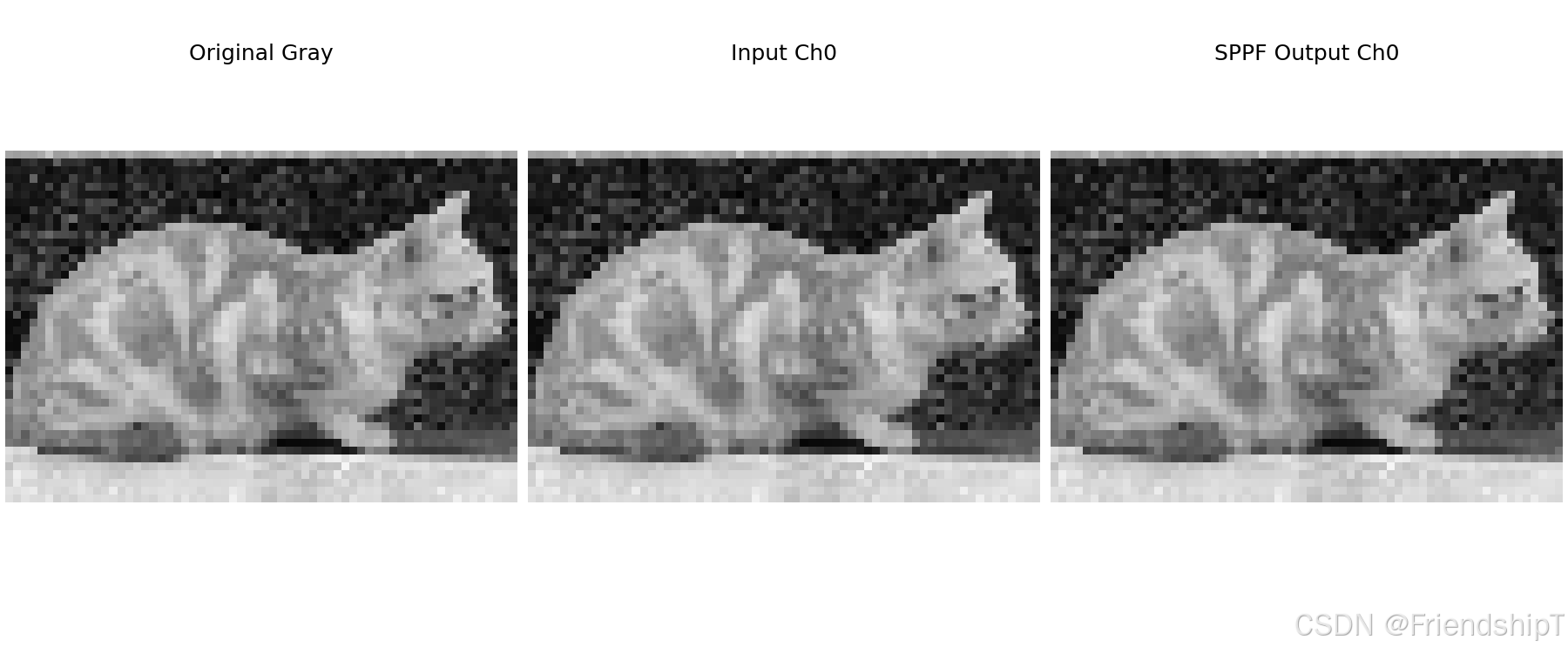
python
if __name__ == '__main__':
    # 1. 随机输入
    x = torch.randn(1, 64, 32, 32)

    # 2. 创建 SPPF(默认 k=5, n=3, shortcut=False)
    sppf = SPPF(c1=64, c2=128, k=5, n=3, shortcut=False)

    # 3. 前向传播
    with torch.no_grad():
        out = sppf(x)
    print("输入形状:", x.shape)   # [1, 64, 32, 32]
    print("输出形状:", out.shape) # [1, 128, 32, 32]

    # 4. 使用真实图像演示(扩展为多通道)
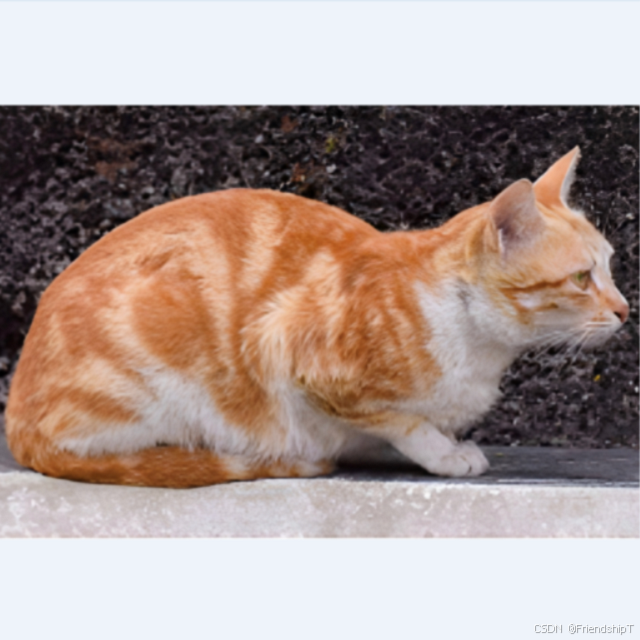
    img_path = "cat_640x640.png"
    img_bgr = cv2.imread(img_path)
    if img_bgr is not None:
        img_gray = cv2.cvtColor(cv2.resize(img_bgr, (64, 64)), cv2.COLOR_BGR2GRAY)
        img_tensor = torch.from_numpy(img_gray).float().unsqueeze(0).unsqueeze(0)  # [1,1,64,64]
        # 扩展通道至64
        x_img = img_tensor.repeat(1, 64, 1, 1)

        sppf_img = SPPF(c1=64, c2=64, k=5, n=3, shortcut=True)
        with torch.no_grad():
            out_img = sppf_img(x_img)

        inp_ch0 = x_img[0, 0].cpu().numpy()
        out_ch0 = out_img[0, 0].cpu().numpy()

        def norm(arr):
            return (arr - arr.min()) / (arr.max() - arr.min() + 1e-8)

        plt.figure(figsize=(12, 5), constrained_layout=True)
        plt.subplot(1, 3, 1)
        plt.imshow(img_gray, cmap='gray')
        plt.title("Original Gray")
        plt.axis("off")
        plt.subplot(1, 3, 2)
        plt.imshow(norm(inp_ch0), cmap='gray')
        plt.title("Input Ch0")
        plt.axis("off")
        plt.subplot(1, 3, 3)
        plt.imshow(norm(out_ch0), cmap='gray')
        plt.title("SPPF Output Ch0")
        plt.axis("off")
        plt.savefig("sppf_demo.png", dpi=150)
print("可视化已保存为 sppf_demo.png")输出示例:
输入形状: torch.Size([1, 64, 32, 32])
输出形状: torch.Size([1, 128, 32, 32])
可视化已保存为 sppf_demo.png
流程示意图
#mermaid-svg-XzcHJxGt2k865Kst{font-family:"trebuchet ms",verdana,arial,sans-serif;font-size:16px;fill:#333;}@keyframes edge-animation-frame{from{stroke-dashoffset:0;}}@keyframes dash{to{stroke-dashoffset:0;}}#mermaid-svg-XzcHJxGt2k865Kst .edge-animation-slow{stroke-dasharray:9,5!important;stroke-dashoffset:900;animation:dash 50s linear infinite;stroke-linecap:round;}#mermaid-svg-XzcHJxGt2k865Kst .edge-animation-fast{stroke-dasharray:9,5!important;stroke-dashoffset:900;animation:dash 20s linear infinite;stroke-linecap:round;}#mermaid-svg-XzcHJxGt2k865Kst .error-icon{fill:#552222;}#mermaid-svg-XzcHJxGt2k865Kst .error-text{fill:#552222;stroke:#552222;}#mermaid-svg-XzcHJxGt2k865Kst .edge-thickness-normal{stroke-width:1px;}#mermaid-svg-XzcHJxGt2k865Kst .edge-thickness-thick{stroke-width:3.5px;}#mermaid-svg-XzcHJxGt2k865Kst .edge-pattern-solid{stroke-dasharray:0;}#mermaid-svg-XzcHJxGt2k865Kst .edge-thickness-invisible{stroke-width:0;fill:none;}#mermaid-svg-XzcHJxGt2k865Kst .edge-pattern-dashed{stroke-dasharray:3;}#mermaid-svg-XzcHJxGt2k865Kst .edge-pattern-dotted{stroke-dasharray:2;}#mermaid-svg-XzcHJxGt2k865Kst .marker{fill:#333333;stroke:#333333;}#mermaid-svg-XzcHJxGt2k865Kst .marker.cross{stroke:#333333;}#mermaid-svg-XzcHJxGt2k865Kst svg{font-family:"trebuchet ms",verdana,arial,sans-serif;font-size:16px;}#mermaid-svg-XzcHJxGt2k865Kst p{margin:0;}#mermaid-svg-XzcHJxGt2k865Kst .label{font-family:"trebuchet ms",verdana,arial,sans-serif;color:#333;}#mermaid-svg-XzcHJxGt2k865Kst .cluster-label text{fill:#333;}#mermaid-svg-XzcHJxGt2k865Kst .cluster-label span{color:#333;}#mermaid-svg-XzcHJxGt2k865Kst .cluster-label span p{background-color:transparent;}#mermaid-svg-XzcHJxGt2k865Kst .label text,#mermaid-svg-XzcHJxGt2k865Kst span{fill:#333;color:#333;}#mermaid-svg-XzcHJxGt2k865Kst .node rect,#mermaid-svg-XzcHJxGt2k865Kst .node circle,#mermaid-svg-XzcHJxGt2k865Kst .node ellipse,#mermaid-svg-XzcHJxGt2k865Kst .node polygon,#mermaid-svg-XzcHJxGt2k865Kst .node path{fill:#ECECFF;stroke:#9370DB;stroke-width:1px;}#mermaid-svg-XzcHJxGt2k865Kst .rough-node .label text,#mermaid-svg-XzcHJxGt2k865Kst .node .label text,#mermaid-svg-XzcHJxGt2k865Kst .image-shape .label,#mermaid-svg-XzcHJxGt2k865Kst .icon-shape .label{text-anchor:middle;}#mermaid-svg-XzcHJxGt2k865Kst .node .katex path{fill:#000;stroke:#000;stroke-width:1px;}#mermaid-svg-XzcHJxGt2k865Kst .rough-node .label,#mermaid-svg-XzcHJxGt2k865Kst .node .label,#mermaid-svg-XzcHJxGt2k865Kst .image-shape .label,#mermaid-svg-XzcHJxGt2k865Kst .icon-shape .label{text-align:center;}#mermaid-svg-XzcHJxGt2k865Kst .node.clickable{cursor:pointer;}#mermaid-svg-XzcHJxGt2k865Kst .root .anchor path{fill:#333333!important;stroke-width:0;stroke:#333333;}#mermaid-svg-XzcHJxGt2k865Kst .arrowheadPath{fill:#333333;}#mermaid-svg-XzcHJxGt2k865Kst .edgePath .path{stroke:#333333;stroke-width:2.0px;}#mermaid-svg-XzcHJxGt2k865Kst .flowchart-link{stroke:#333333;fill:none;}#mermaid-svg-XzcHJxGt2k865Kst .edgeLabel{background-color:rgba(232,232,232, 0.8);text-align:center;}#mermaid-svg-XzcHJxGt2k865Kst .edgeLabel p{background-color:rgba(232,232,232, 0.8);}#mermaid-svg-XzcHJxGt2k865Kst .edgeLabel rect{opacity:0.5;background-color:rgba(232,232,232, 0.8);fill:rgba(232,232,232, 0.8);}#mermaid-svg-XzcHJxGt2k865Kst .labelBkg{background-color:rgba(232, 232, 232, 0.5);}#mermaid-svg-XzcHJxGt2k865Kst .cluster rect{fill:#ffffde;stroke:#aaaa33;stroke-width:1px;}#mermaid-svg-XzcHJxGt2k865Kst .cluster text{fill:#333;}#mermaid-svg-XzcHJxGt2k865Kst .cluster span{color:#333;}#mermaid-svg-XzcHJxGt2k865Kst div.mermaidTooltip{position:absolute;text-align:center;max-width:200px;padding:2px;font-family:"trebuchet ms",verdana,arial,sans-serif;font-size:12px;background:hsl(80, 100%, 96.2745098039%);border:1px solid #aaaa33;border-radius:2px;pointer-events:none;z-index:100;}#mermaid-svg-XzcHJxGt2k865Kst .flowchartTitleText{text-anchor:middle;font-size:18px;fill:#333;}#mermaid-svg-XzcHJxGt2k865Kst rect.text{fill:none;stroke-width:0;}#mermaid-svg-XzcHJxGt2k865Kst .icon-shape,#mermaid-svg-XzcHJxGt2k865Kst .image-shape{background-color:rgba(232,232,232, 0.8);text-align:center;}#mermaid-svg-XzcHJxGt2k865Kst .icon-shape p,#mermaid-svg-XzcHJxGt2k865Kst .image-shape p{background-color:rgba(232,232,232, 0.8);padding:2px;}#mermaid-svg-XzcHJxGt2k865Kst .icon-shape .label rect,#mermaid-svg-XzcHJxGt2k865Kst .image-shape .label rect{opacity:0.5;background-color:rgba(232,232,232, 0.8);fill:rgba(232,232,232, 0.8);}#mermaid-svg-XzcHJxGt2k865Kst .label-icon{display:inline-block;height:1em;overflow:visible;vertical-align:-0.125em;}#mermaid-svg-XzcHJxGt2k865Kst .node .label-icon path{fill:currentColor;stroke:revert;stroke-width:revert;}#mermaid-svg-XzcHJxGt2k865Kst :root{--mermaid-font-family:"trebuchet ms",verdana,arial,sans-serif;} 是
否
输入 x (B, c1, H, W)
Conv 1x1: c1 -> c_ (cv1, act=False)
原始特征 (B, c_, H, W)
MaxPool2d kxk, stride=1, padding=k//2
池化结果1
MaxPool2d kxk
池化结果2
... 重复 n 次
池化结果n
拼接 (沿通道维): 原始, 结果1, ..., 结果n
Conv 1x1: c_*(n+1) -> c2 (cv2)
shortcut=True 且 c1==c2?
残差相加: 输出 + 输入
直接输出
输出 (B, c2, H, W)
代码解读
__init__:c_ = c1 // 2:隐藏通道数。self.cv1:1×1 卷积,act=False,即不包含激活函数(仅 Conv+BN),用于通道降维。self.cv2:1×1 卷积,act默认 True(SiLU),用于将拼接后的高维特征压缩至c2。self.m:单层最大池化,核大小为k,步长 1,填充k//2,保持空间分辨率。self.n:池化次数。self.add:布尔值,标记是否启用残差连接。
forward:y = [self.cv1(x)]:存储降维后的特征。- 循环
n次,每次对y[-1]进行池化,并将结果追加到y。 - 拼接所有
y元素。 - 通过
cv2压缩。 - 若
self.add为真,则加上原始输入x,否则直接返回。
与 SPP 的对比
| 特性 | SPP | SPPF |
|---|---|---|
| 实现方式 | 并行多核池化(如 5,9,13) | 串联单核池化(多次 5×5) |
| 计算量 | 较高,需同时执行多个池化 | 较低,仅一个池化层重复使用 |
| 感受野等效 | 直接使用不同核大小 | 等效感受野:k, 2k-1, 3k-2(k=5 → 5,9,13) |
| 内存占用 | 需存储多个池化结果 | 需存储中间结果,但随 n 可调 |
| 速度 | 较慢 | 较快(约快 2 倍) |
注意事项
- 空间尺寸不变 :池化
stride=1且padding=k//2,保持 H、W 不变。 - 通道数变化 :输入通道先减半,拼接后通道数增加,最终压缩到
c2。 act=False的影响 :cv1无激活,可能减少非线性,但后续拼接和cv2的激活可弥补。shortcut条件 :残差连接仅在c1 == c2时生效,且需设置shortcut=True。- 等效性验证 :
SPPF(k=5, n=3)与SPP(k=(5,9,13))理论上等价,但实际可能有微小差异(由于池化串联的非线性性质),但实验证明效果相近且速度更快。
优缺点
优点
- 计算高效:相比 SPP,减少了池化操作的次数,显著提升推理速度。
- 轻量级:仅需一个池化层,参数更少。
- 等效感受野:通过串联池化获得类似多核池化的效果,保持多尺度能力。
- 灵活可调 :通过
k和n可控制感受野范围和计算量。 - 残差选项:可选的 shortcut 有助于梯度流动。
缺点
- 非线性累积:串联池化可能引入更多非线性,导致特征分布改变,但通常影响微小。
- 等效性并非完全等价:串联池化与并行池化在数学上不完全等价,但在实践中效果良好。
- 对
n的选择敏感 :n过小感受野不足,过大则计算量增加且可能冗余。 - 无内置多种核选择:只能使用单一核大小,灵活性略低于 SPP。
在 YOLOv5/v8 等网络中,SPPF 已成为标准配置,取代了原始的 SPP。实际使用时,通常采用默认参数 k=5, n=3,并可根据硬件资源调整 n 以平衡速度与性能。
SPP 与 SPPF 的区别
SPP 和 SPPF 都是空间金字塔池化模块,用于在保持空间分辨率的同时聚合多尺度上下文信息。二者的核心区别在于 实现方式:
- SPP(Spatial Pyramid Pooling) :使用 多个不同尺寸的池化核 (如 5×5、9×9、13×13)并行地对输入特征图进行最大池化,然后将原始特征与所有池化结果在通道维拼接。这种方式能直接获得不同感受野的特征,但计算开销较大。
- SPPF(Spatial Pyramid Pooling - Fast) :使用 单个小尺寸池化核 (如 5×5)串联地多次池化(默认 3 次),每次池化输出作为下一次的输入,并将原始特征与每次池化后的结果拼接。通过串联,可以等效地获得与 SPP 相似的多尺度感受野(对于 k=5, n=3,等效感受野为 5、9、13),但计算量显著降低,速度更快。
结构对比图
#mermaid-svg-ICtlYwI2UIvOTzaB{font-family:"trebuchet ms",verdana,arial,sans-serif;font-size:16px;fill:#333;}@keyframes edge-animation-frame{from{stroke-dashoffset:0;}}@keyframes dash{to{stroke-dashoffset:0;}}#mermaid-svg-ICtlYwI2UIvOTzaB .edge-animation-slow{stroke-dasharray:9,5!important;stroke-dashoffset:900;animation:dash 50s linear infinite;stroke-linecap:round;}#mermaid-svg-ICtlYwI2UIvOTzaB .edge-animation-fast{stroke-dasharray:9,5!important;stroke-dashoffset:900;animation:dash 20s linear infinite;stroke-linecap:round;}#mermaid-svg-ICtlYwI2UIvOTzaB .error-icon{fill:#552222;}#mermaid-svg-ICtlYwI2UIvOTzaB .error-text{fill:#552222;stroke:#552222;}#mermaid-svg-ICtlYwI2UIvOTzaB .edge-thickness-normal{stroke-width:1px;}#mermaid-svg-ICtlYwI2UIvOTzaB .edge-thickness-thick{stroke-width:3.5px;}#mermaid-svg-ICtlYwI2UIvOTzaB .edge-pattern-solid{stroke-dasharray:0;}#mermaid-svg-ICtlYwI2UIvOTzaB .edge-thickness-invisible{stroke-width:0;fill:none;}#mermaid-svg-ICtlYwI2UIvOTzaB .edge-pattern-dashed{stroke-dasharray:3;}#mermaid-svg-ICtlYwI2UIvOTzaB .edge-pattern-dotted{stroke-dasharray:2;}#mermaid-svg-ICtlYwI2UIvOTzaB .marker{fill:#333333;stroke:#333333;}#mermaid-svg-ICtlYwI2UIvOTzaB .marker.cross{stroke:#333333;}#mermaid-svg-ICtlYwI2UIvOTzaB svg{font-family:"trebuchet ms",verdana,arial,sans-serif;font-size:16px;}#mermaid-svg-ICtlYwI2UIvOTzaB p{margin:0;}#mermaid-svg-ICtlYwI2UIvOTzaB .label{font-family:"trebuchet ms",verdana,arial,sans-serif;color:#333;}#mermaid-svg-ICtlYwI2UIvOTzaB .cluster-label text{fill:#333;}#mermaid-svg-ICtlYwI2UIvOTzaB .cluster-label span{color:#333;}#mermaid-svg-ICtlYwI2UIvOTzaB .cluster-label span p{background-color:transparent;}#mermaid-svg-ICtlYwI2UIvOTzaB .label text,#mermaid-svg-ICtlYwI2UIvOTzaB span{fill:#333;color:#333;}#mermaid-svg-ICtlYwI2UIvOTzaB .node rect,#mermaid-svg-ICtlYwI2UIvOTzaB .node circle,#mermaid-svg-ICtlYwI2UIvOTzaB .node ellipse,#mermaid-svg-ICtlYwI2UIvOTzaB .node polygon,#mermaid-svg-ICtlYwI2UIvOTzaB .node path{fill:#ECECFF;stroke:#9370DB;stroke-width:1px;}#mermaid-svg-ICtlYwI2UIvOTzaB .rough-node .label text,#mermaid-svg-ICtlYwI2UIvOTzaB .node .label text,#mermaid-svg-ICtlYwI2UIvOTzaB .image-shape .label,#mermaid-svg-ICtlYwI2UIvOTzaB .icon-shape .label{text-anchor:middle;}#mermaid-svg-ICtlYwI2UIvOTzaB .node .katex path{fill:#000;stroke:#000;stroke-width:1px;}#mermaid-svg-ICtlYwI2UIvOTzaB .rough-node .label,#mermaid-svg-ICtlYwI2UIvOTzaB .node .label,#mermaid-svg-ICtlYwI2UIvOTzaB .image-shape .label,#mermaid-svg-ICtlYwI2UIvOTzaB .icon-shape .label{text-align:center;}#mermaid-svg-ICtlYwI2UIvOTzaB .node.clickable{cursor:pointer;}#mermaid-svg-ICtlYwI2UIvOTzaB .root .anchor path{fill:#333333!important;stroke-width:0;stroke:#333333;}#mermaid-svg-ICtlYwI2UIvOTzaB .arrowheadPath{fill:#333333;}#mermaid-svg-ICtlYwI2UIvOTzaB .edgePath .path{stroke:#333333;stroke-width:2.0px;}#mermaid-svg-ICtlYwI2UIvOTzaB .flowchart-link{stroke:#333333;fill:none;}#mermaid-svg-ICtlYwI2UIvOTzaB .edgeLabel{background-color:rgba(232,232,232, 0.8);text-align:center;}#mermaid-svg-ICtlYwI2UIvOTzaB .edgeLabel p{background-color:rgba(232,232,232, 0.8);}#mermaid-svg-ICtlYwI2UIvOTzaB .edgeLabel rect{opacity:0.5;background-color:rgba(232,232,232, 0.8);fill:rgba(232,232,232, 0.8);}#mermaid-svg-ICtlYwI2UIvOTzaB .labelBkg{background-color:rgba(232, 232, 232, 0.5);}#mermaid-svg-ICtlYwI2UIvOTzaB .cluster rect{fill:#ffffde;stroke:#aaaa33;stroke-width:1px;}#mermaid-svg-ICtlYwI2UIvOTzaB .cluster text{fill:#333;}#mermaid-svg-ICtlYwI2UIvOTzaB .cluster span{color:#333;}#mermaid-svg-ICtlYwI2UIvOTzaB div.mermaidTooltip{position:absolute;text-align:center;max-width:200px;padding:2px;font-family:"trebuchet ms",verdana,arial,sans-serif;font-size:12px;background:hsl(80, 100%, 96.2745098039%);border:1px solid #aaaa33;border-radius:2px;pointer-events:none;z-index:100;}#mermaid-svg-ICtlYwI2UIvOTzaB .flowchartTitleText{text-anchor:middle;font-size:18px;fill:#333;}#mermaid-svg-ICtlYwI2UIvOTzaB rect.text{fill:none;stroke-width:0;}#mermaid-svg-ICtlYwI2UIvOTzaB .icon-shape,#mermaid-svg-ICtlYwI2UIvOTzaB .image-shape{background-color:rgba(232,232,232, 0.8);text-align:center;}#mermaid-svg-ICtlYwI2UIvOTzaB .icon-shape p,#mermaid-svg-ICtlYwI2UIvOTzaB .image-shape p{background-color:rgba(232,232,232, 0.8);padding:2px;}#mermaid-svg-ICtlYwI2UIvOTzaB .icon-shape .label rect,#mermaid-svg-ICtlYwI2UIvOTzaB .image-shape .label rect{opacity:0.5;background-color:rgba(232,232,232, 0.8);fill:rgba(232,232,232, 0.8);}#mermaid-svg-ICtlYwI2UIvOTzaB .label-icon{display:inline-block;height:1em;overflow:visible;vertical-align:-0.125em;}#mermaid-svg-ICtlYwI2UIvOTzaB .node .label-icon path{fill:currentColor;stroke:revert;stroke-width:revert;}#mermaid-svg-ICtlYwI2UIvOTzaB :root{--mermaid-font-family:"trebuchet ms",verdana,arial,sans-serif;} SPPF (串联单核)
输入 x
Conv 1x1 降维
原始特征
MaxPool k=5 (第1次)
MaxPool k=5 (第2次)
MaxPool k=5 (第3次)
拼接 (通道维)
Conv 1x1 输出
SPP (并行多核)
输入 x
Conv 1x1 降维
原始特征
MaxPool k1=5
MaxPool k2=9
MaxPool k3=13
拼接 (通道维)
Conv 1x1 输出
对比表格
| 特性 | SPP | SPPF |
|---|---|---|
| 池化方式 | 并行,多个不同核 | 串联,同一核多次 |
| 核大小 | 如 (5, 9, 13) | 通常 5×5,重复 3 次 |
| 等效感受野 | 直接由各核决定 | k, 2k-1, 3k-2(k=5 → 5, 9, 13) |
| 计算量 | 较高(多个池化层) | 较低(单池化层重复) |
| 推理速度 | 较慢 | 较快(约 2 倍加速) |
| 数学等价性 | 标准实现 | 近似等价,实践中效果相近 |
| 典型用途 | YOLOv5 早期版本 | YOLOv5/v8 标准配置 |
| 内存占用 | 较高(需存储多个结果) | 较低(仅存储中间结果) |
总结
SPPF 通过串联小核池化,以更低的计算成本获得了与 SPP 相似的多尺度特征聚合能力,因此在现代 YOLO 系列中被广泛采用(YOLOv5、YOLOv8 等)。若硬件资源充足且对精度有极致要求,可尝试 SPP;若追求效率优先,SPPF 是更优选择。
参考文献
1 https://docs.ultralytics.com/
2 https://github.com/ultralytics/ultralytics.git
- 由于本人水平有限,难免出现错漏,敬请批评改正。
- 更多精彩内容,可点击进入Python日常小操作专栏、OpenCV-Python小应用专栏、YOLO系列专栏、自然语言处理专栏、人工智能混合编程实践专栏或我的个人主页查看
- YOLOs-CPP:一个免费开源的YOLO全系列C++推理库(以YOLO26为例)
- PaddleOCR:Win10上安装使用PPOCRLabel标注工具
- 目标检测:使用自己的数据集微调DEIMv2进行物体检测
- 图像分割:PyTorch从零开始实现SegFormer语义分割
- 图像超分:使用自己的数据集微调Real-ESRGAN-x4plus进行超分重建
- 图像生成:PyTorch从零开始实现一个简单的扩散模型
- Stable Diffusion:使用自己的数据集微调 Stable Diffusion 3.5 LoRA 文生图模型
- 图像超分:使用自己的数据集微调Real-ESRGAN-x2plus进行超分重建
- Anomalib:使用Anomalib 2.1.0训练自己的数据集进行异常检测
- Anomalib:在Linux服务器上安装使用Anomalib 2.1.0
- 人工智能混合编程实践:C++调用封装好的DLL进行异常检测推理
- 人工智能混合编程实践:C++调用封装好的DLL进行FP16图像超分重建(v3.0)
- 隔离系统Python:源码编译3.11.8到自定义目录(含PGO性能优化)
- 在线机的Python环境迁移到离线机上
- Nuitka 将 Python 脚本封装为 .pyd 或 .so 文件
- Ultralytics:使用 YOLO11 进行速度估计
- Ultralytics:使用 YOLO11 进行物体追踪
- Ultralytics:使用 YOLO11 进行物体计数
- Ultralytics:使用 YOLO11 进行目标打码
- 人工智能混合编程实践:C++调用Python ONNX进行YOLOv8推理
- 人工智能混合编程实践:C++调用封装好的DLL进行YOLOv8实例分割
- 人工智能混合编程实践:C++调用Python ONNX进行图像超分重建
- 人工智能混合编程实践:C++调用Python AgentOCR进行文本识别
- 通过计算实例简单地理解PatchCore异常检测
- Python将YOLO格式实例分割数据集转换为COCO格式实例分割数据集
- YOLOv8 Ultralytics:使用Ultralytics框架训练RT-DETR实时目标检测模型
- 基于DETR的人脸伪装检测
- YOLOv7训练自己的数据集(口罩检测)
- YOLOv8训练自己的数据集(足球检测)
- YOLOv5:TensorRT加速YOLOv5模型推理
- YOLOv5:IoU、GIoU、DIoU、CIoU、EIoU
- 玩转Jetson Nano(五):TensorRT加速YOLOv5目标检测
- YOLOv5:添加SE、CBAM、CoordAtt、ECA注意力机制
- YOLOv5:yolov5s.yaml配置文件解读、增加小目标检测层
- Python将COCO格式实例分割数据集转换为YOLO格式实例分割数据集
- YOLOv5:使用7.0版本训练自己的实例分割模型(车辆、行人、路标、车道线等实例分割)
- 使用Kaggle GPU资源免费体验Stable Diffusion开源项目
- Stable Diffusion:在服务器上部署使用Stable Diffusion WebUI进行AI绘图(v2.0)
- Stable Diffusion:使用自己的数据集微调训练LoRA模型(v2.0)