数据集为NASA锂电池数据集。
import datetimeimport numpy as npimport pandas as pdfrom scipy.io import loadmatfrom sklearn.preprocessing import MinMaxScalerfrom sklearn.metrics import mean_squared_errorfrom sklearn import metricsimport matplotlib.pyplot as pltimport seaborn as snsLoad Dataset
def load_data(battery): mat = loadmat('' + battery + '.mat') print('Total data in dataset: ', len(mat[battery][0, 0]['cycle'][0])) counter = 0 dataset = [] capacity_data = [] for i in range(len(mat[battery][0, 0]['cycle'][0])): row = mat[battery][0, 0]['cycle'][0, i] if row['type'][0] == 'discharge': ambient_temperature = row['ambient_temperature'][0][0] date_time = datetime.datetime(int(row['time'][0][0]), int(row['time'][0][1]), int(row['time'][0][2]), int(row['time'][0][3]), int(row['time'][0][4])) + datetime.timedelta(seconds=int(row['time'][0][5])) data = row['data'] capacity = data[0][0]['Capacity'][0][0] for j in range(len(data[0][0]['Voltage_measured'][0])): voltage_measured = data[0][0]['Voltage_measured'][0][j] current_measured = data[0][0]['Current_measured'][0][j] temperature_measured = data[0][0]['Temperature_measured'][0][j] current_load = data[0][0]['Current_load'][0][j] voltage_load = data[0][0]['Voltage_load'][0][j] time = data[0][0]['Time'][0][j] dataset.append([counter + 1, ambient_temperature, date_time, capacity, voltage_measured, current_measured, temperature_measured, current_load, voltage_load, time]) capacity_data.append([counter + 1, ambient_temperature, date_time, capacity]) counter = counter + 1 print(dataset[0]) return [pd.DataFrame(data=dataset, columns=['cycle', 'ambient_temperature', 'datetime', 'capacity', 'voltage_measured', 'current_measured', 'temperature_measured', 'current_load', 'voltage_load', 'time']), pd.DataFrame(data=capacity_data, columns=['cycle', 'ambient_temperature', 'datetime', 'capacity'])]dataset, capacity = load_data('B0005')pd.set_option('display.max_columns', 10)Total data in dataset: 616
[1, 24, datetime.datetime(2008, 4, 2, 15, 25, 41), 1.8564874208181574, 4.191491807505295, -0.004901589207462691, 24.330033885570543, -0.0006, 0.0, 0.0]dataset.head()
plot_df = capacity.loc[(capacity['cycle']>=1),['cycle','capacity']]sns.set_style("darkgrid")plt.figure(figsize=(12, 8))plt.plot(plot_df['cycle'], plot_df['capacity'])#Draw thresholdplt.plot([0.,len(capacity)], [1.4, 1.4])plt.ylabel('Capacity')# make x-axis ticks legibleadf = plt.gca().get_xaxis().get_major_formatter()plt.xlabel('cycle')plt.title('Discharge B0005')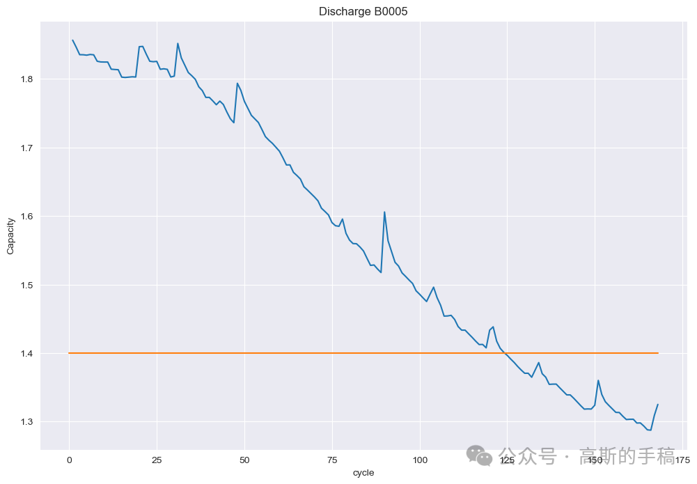
plot_df = dis_ele.loc[(dis_ele['cycle']>=1),['cycle','SoH']]sns.set_style("white")plt.figure(figsize=(8, 5))plt.plot(plot_df['cycle'], plot_df['SoH'])#Draw thresholdplt.plot([0.,len(capacity)], [0.70, 0.70])plt.ylabel('SOH')# make x-axis ticks legibleadf = plt.gca().get_xaxis().get_major_formatter()plt.xlabel('cycle')plt.title('Discharge B0005')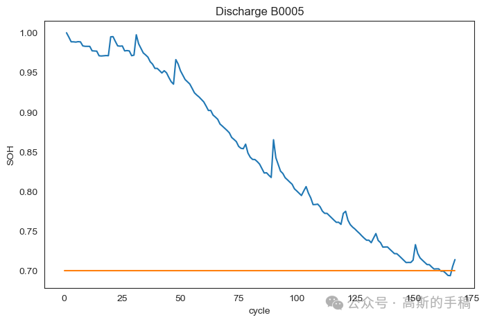
cycle_array= np.array(dataset['cycle'])dataset['RUL'] = 168-cycle_arraydataset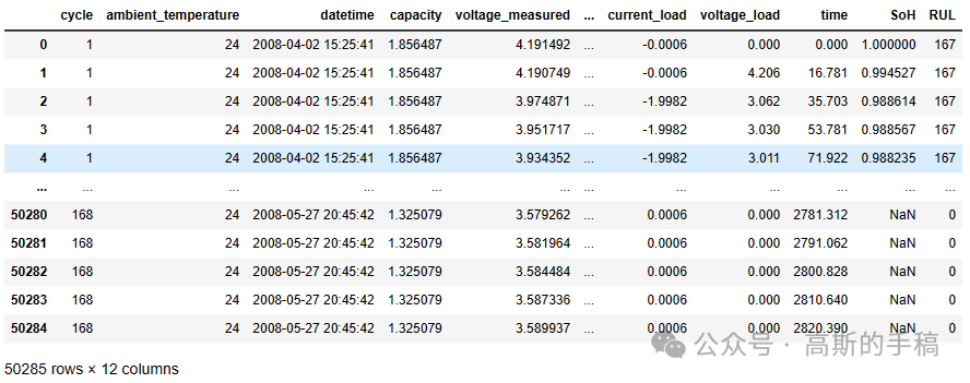
df = datasetdf = df.drop(columns = ['SoH'])Explodatory Data Analysis
df.head()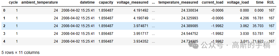
df.describe()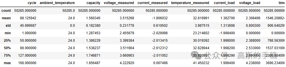
sns.heatmap(df.corr(), annot = True)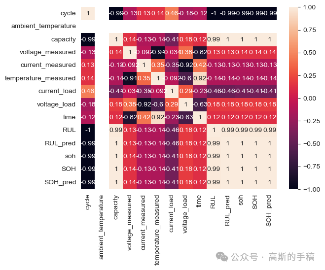
df.info()<class 'pandas.core.frame.DataFrame'>
RangeIndex: 50285 entries, 0 to 50284
Data columns (total 12 columns):
# Column Non-Null Count Dtype
--- ------ -------------- -----
0 cycle 50285 non-null int64
1 ambient_temperature 50285 non-null int32
2 datetime 50285 non-null datetime64[ns]
3 capacity 50285 non-null float64
4 voltage_measured 50285 non-null float64
5 current_measured 50285 non-null float64
6 temperature_measured 50285 non-null float64
7 current_load 50285 non-null float64
8 voltage_load 50285 non-null float64
9 time 50285 non-null float64
10 RUL 50285 non-null int64
11 SOH 50285 non-null float64
dtypes: datetime64[ns](1), float64(8), int32(1), int64(2)
memory usage: 4.4 MBdataset.isna().sum()cycle 0
ambient_temperature 0
datetime 0
capacity 0
voltage_measured 0
current_measured 0
temperature_measured 0
current_load 0
voltage_load 0
time 0
SoH 50117dtype: int64
Machine learning Implementation
from sklearn.model_selection import train_test_splitfrom sklearn.linear_model import LinearRegressionfrom sklearn.tree import DecisionTreeRegressorfrom sklearn.ensemble import RandomForestRegressorfrom sklearn.metrics import mean_squared_error, r2_scoreimport pandas as pd
# Assuming df is your DataFramefeatures = ['cycle', 'ambient_temperature', 'voltage_measured', 'current_measured', 'temperature_measured', 'current_load', 'voltage_load', 'time']target = 'SOH'
# Split the data into features (X) and target variable (y)X = df[features]y = df[target]
# Train-test splitX_train, X_test, y_train, y_test = train_test_split(X, y, test_size=0.2, random_state=42)
# Linear Regressionlinear_model = LinearRegression()linear_model.fit(X_train, y_train)linear_predictions = linear_model.predict(X_test)
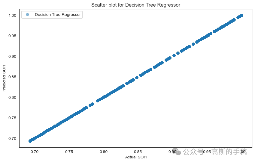
# Decision Tree Regressordt_model = DecisionTreeRegressor(random_state=42)dt_model.fit(X_train, y_train)dt_predictions = dt_model.predict(X_test)
# Random Forest Regressorrf_model = RandomForestRegressor(random_state=42)rf_model.fit(X_train, y_train)rf_predictions = rf_model.predict(X_test)
# Evaluate the modelsdef evaluate_model(predictions, y_test, model_name):    mse = mean_squared_error(y_test, predictions)    r2 = r2_score(y_test, predictions)    print(f"{model_name} - Mean Squared Error: {mse}, R-squared: {r2}")
evaluate_model(linear_predictions, y_test, 'Linear Regression')evaluate_model(dt_predictions, y_test, 'Decision Tree Regressor')evaluate_model(rf_predictions, y_test, 'Random Forest Regressor')Linear Regression - Mean Squared Error: 0.0002239971272592741, R-squared: 0.9768123399683541
Decision Tree Regressor - Mean Squared Error: 5.793947345542318e-30, R-squared: 1.0
Random Forest Regressor - Mean Squared Error: 1.2263587861112884e-09, R-squared: 0.9999998730501996Ensemble techniques
from sklearn.ensemble import BaggingRegressor, GradientBoostingRegressorfrom sklearn.metrics import mean_squared_error, r2_scorefrom sklearn.model_selection import train_test_splitimport pandas as pd
# Assuming df is your DataFramefeatures = ['cycle', 'ambient_temperature', 'voltage_measured', 'current_measured', 'temperature_measured', 'current_load', 'voltage_load', 'time']target = 'SOH'
# Split the data into features (X) and target variable (y)X = df[features]y = df[target]
# Train-test splitX_train, X_test, y_train, y_test = train_test_split(X, y, test_size=0.2, random_state=42)
# Bagging with Random Forestbagging_model = BaggingRegressor(base_estimator=RandomForestRegressor(), n_estimators=10, random_state=42)bagging_model.fit(X_train, y_train)bagging_predictions = bagging_model.predict(X_test)
# Boosting with Gradient Boostingboosting_model = GradientBoostingRegressor(n_estimators=100, learning_rate=0.1, random_state=42)boosting_model.fit(X_train, y_train)boosting_predictions = boosting_model.predict(X_test)
# Evaluate the modelsdef evaluate_model(predictions, y_test, model_name):    mse = mean_squared_error(y_test, predictions)    r2 = r2_score(y_test, predictions)    print(f"{model_name} - Mean Squared Error: {mse}, R-squared: {r2}")
evaluate_model(bagging_predictions, y_test, 'Bagging with Random Forest')evaluate_model(boosting_predictions, y_test, 'Boosting with Gradient Boosting')Bagging with Random Forest - Mean Squared Error: 1.076830712151592e-11, R-squared: 0.99999999888529
Boosting with Gradient Boosting - Mean Squared Error: 3.0152836389704887e-06, R-squared: 0.9996878648723093Visualize the predicted values against the actual values
import matplotlib.pyplot as pltimport numpy as np
# Scatter plot for Linear Regressionplt.figure(figsize=(10, 6))plt.scatter(y_test, linear_predictions, label='Linear Regression', alpha=0.5)plt.xlabel('Actual SOH')plt.ylabel('Predicted SOH')plt.title('Scatter plot for Linear Regression')plt.legend()plt.show()
# Scatter plot for Decision Tree Regressorplt.figure(figsize=(10, 6))plt.scatter(y_test, dt_predictions, label='Decision Tree Regressor', alpha=0.5)plt.xlabel('Actual SOH')plt.ylabel('Predicted SOH')plt.title('Scatter plot for Decision Tree Regressor')plt.legend()plt.show()
# Scatter plot for Random Forest Regressorplt.figure(figsize=(10, 6))plt.scatter(y_test, rf_predictions, label='Random Forest Regressor', alpha=0.5)plt.xlabel('Actual SOH')plt.ylabel('Predicted SOH')plt.title('Scatter plot for Random Forest Regressor')plt.legend()plt.show()
# Scatter plot for Bagging with Random Forestplt.figure(figsize=(10, 6))plt.scatter(y_test, bagging_predictions, label='Bagging with Random Forest', alpha=0.5)plt.xlabel('Actual SOH')plt.ylabel('Predicted SOH')plt.title('Scatter plot for Bagging with Random Forest')plt.legend()plt.show()
# Scatter plot for Boosting with Gradient Boostingplt.figure(figsize=(10, 6))plt.scatter(y_test, boosting_predictions, label='Boosting with Gradient Boosting', alpha=0.5)plt.xlabel('Actual SOH')plt.ylabel('Predicted SOH')plt.title('Scatter plot for Boosting with Gradient Boosting')plt.legend()plt.show()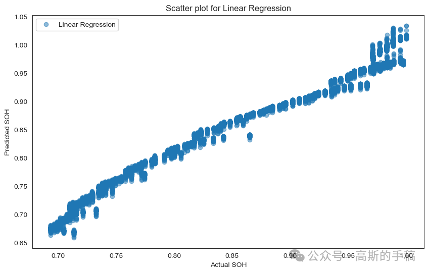
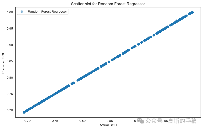
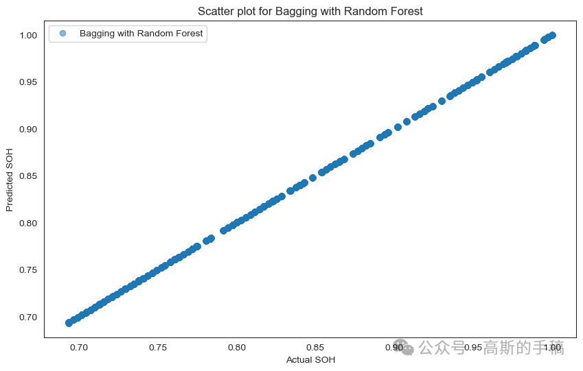
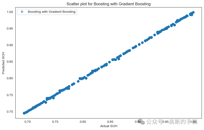
Comparing the accuracy of different models
import matplotlib.pyplot as plt
# R-squared values for each modelr_squared_values = [linear_model.score(X_test, y_test),                    dt_model.score(X_test, y_test),                    rf_model.score(X_test, y_test),                    bagging_model.score(X_test, y_test),                    boosting_model.score(X_test, y_test)]
# Model namesmodel_names = ['Linear Regression', 'Decision Tree', 'Random Forest', 'Bagging with RF', 'Boosting with GB']
# Bar plotplt.figure(figsize=(10, 6))plt.bar(model_names, r_squared_values, color=['blue', 'green', 'orange', 'red', 'purple'])plt.ylabel('R-squared Value')plt.title('R-squared Comparison of Regression Models')plt.ylim(0, 1)  # Set y-axis limit to be between 0 and 1plt.show()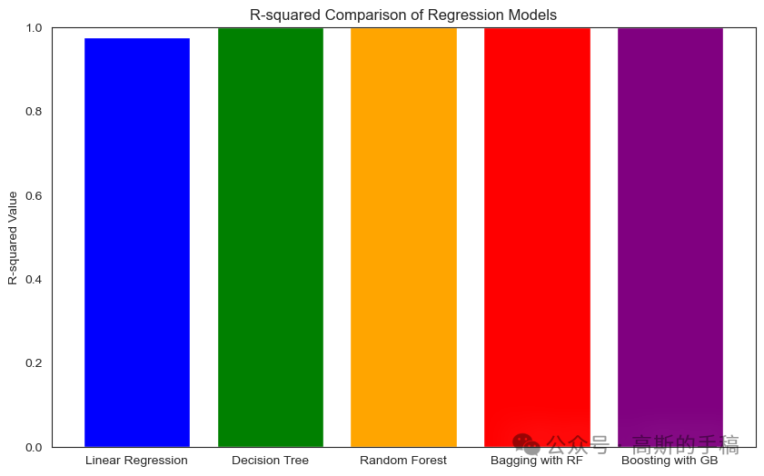
工学博士,担任《Mechanical System and Signal Processing》《中国电机工程学报》《控制与决策》等期刊审稿专家,擅长领域:现代信号处理,机器学习,深度学习,数字孪生,时间序列分析,设备缺陷检测、设备异常检测、设备智能故障诊断与健康管理PHM等。