import numpy as np
import pandas as pd
import matplotlib.pyplot as plt
import plotly.express as px
from sklearn.preprocessing import MinMaxScaler
from sklearn.model_selection import train_test_split
from sklearn.metrics import mean_absolute_percentage_error
import tensorflow as tf
from keras import Model
from keras.layers import Input, Dense, Dropout, LSTM
df = pd.read_csv('Gold Price (2013-2023).csv' )
df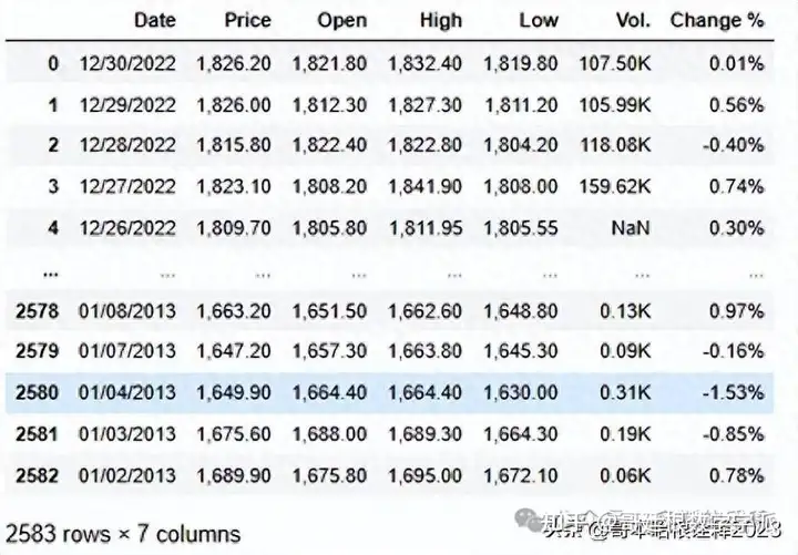
df.info()
<class 'pandas.core.frame.DataFrame'>
RangeIndex: 2583 entries, 0 to 2582
Data columns (total 7 columns):
 #   Column    Non-Null Count  Dtype
---  ------    --------------  -----
 0   Date      2583 non-null   object
 1   Price     2583 non-null   object
 2   Open      2583 non-null   object
 3   High      2583 non-null   object
 4   Low       2583 non-null   object
 5   Vol.      2578 non-null   object
 6   Change %  2583 non-null   object
dtypes: object(7)
memory usage: 141.4+ KB
df.drop(['Vol.', 'Change %'], axis=1, inplace=True)
df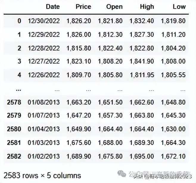
# Convert the 'Date' column to datetime
df['Date'] = pd.to_datetime(df['Date'])


# Sort the DataFrame by the 'Date' column in ascending order
df.sort_values(by='Date', ascending=True, inplace=True)


# Reset the index of the DataFrame
df.reset_index(drop=True, inplace=True)
numCols = df.columns.drop('Date')
df[numCols] = df[numCols].replace({',': ''}, regex=True)
df[numCols] = df[numCols].astype('float64')
df.head()
df.duplicated().sum()
df.isnull().sum()
Date     0
Price    0
Open     0
High     0
Low      0
dtype: int64
import plotly.express as px


fig = px.line(y=df['Price'], x=df['Date'])
fig.update_traces(line_color='black')
fig.update_layout(
    xaxis_title='Date',
    yaxis_title='Price',
    title={
        'text': 'Gold Price Data',
        'y': 0.95,
        'x': 0.5,
        'xanchor': 'center',
        'yanchor': 'top'
    },
    plot_bgcolor='rgba(255,223,0,0.9)'
)
fig.show()
test_size = df[df.Date.dt.year == 2022].shape[0]
print(test_size)
260
import matplotlib.pyplot as plt


plt.figure(figsize=(15, 6), dpi=150)
plt.rcParams['axes.facecolor'] = 'cyan'
plt.rc('axes', edgecolor='white')


plt.plot(df.Date[:-test_size], df.Price[:-test_size], color='black', lw=2)
plt.plot(df.Date[-test_size:], df.Price[-test_size:], color='red', lw=2)


plt.title('Gold Price Train and Test', fontsize=15)
plt.xlabel('Date', fontsize=12)
plt.ylabel('Price', fontsize=12)
plt.legend(['Train Set', 'Test Set'], loc='upper left', prop={'size': 15})
plt.grid(color='white')


plt.show()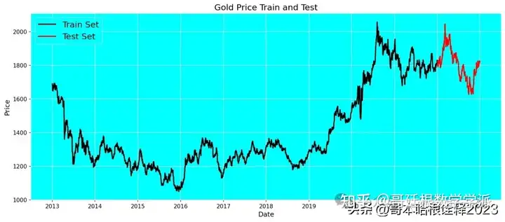
scaler = MinMaxScaler()
scaler.fit(df.Price.values.reshape(-1, 1))
MinMaxScaler()
window_size = 60
train_data = df.Price[:-test_size]
train_data = scaler.fit_transform(train_data.values.reshape(-1, 1))
window_size = 60
X_train = []
y_train = []


for i in range(window_size, len(train_data)):
    X_train.append(train_data[i-window_size:i, 0])
    y_train.append(train_data[i, 0])
test_data = df.Price[-test_size-window_size:]
test_data = scaler.transform(test_data.values.reshape(-1, 1))
X_test = []
y_test = []


for i in range(window_size, len(test_data)):
    X_test.append(test_data[i-window_size:i, 0])
    y_test.append(test_data[i, 0])
X_train = np.array(X_train)
X_test = np.array(X_test)
y_train = np.array(y_train)
y_test = np.array(y_test)


X_train = np.reshape(X_train, (X_train.shape[0], X_train.shape[1], 1))
X_test = np.reshape(X_test, (X_test.shape[0], X_test.shape[1], 1))
y_train = np.reshape(y_train, (-1, 1))
y_test = np.reshape(y_test, (-1, 1))
print('X_train shape:', X_train.shape)
print('y_train shape:', y_train.shape)
print('X_test shape:', X_test.shape)
print('y_test shape:', y_test.shape)
X_train shape: (2263, 60, 1)
y_train shape: (2263, 1)
X_test shape: (260, 60, 1)
y_test shape: (260, 1)
import tensorflow as tf


def define_model():
    input1 = Input(shape=(window_size, 1))
    x = tf.keras.layers.LSTM(units=64, return_sequences=True)(input1)
    x = tf.keras.layers.Dropout(0.2)(x)
    x = tf.keras.layers.LSTM(units=64, return_sequences=True)(x)
    x = tf.keras.layers.Dropout(0.2)(x)
    x = tf.keras.layers.LSTM(units=64)(x)
    x = tf.keras.layers.Dropout(0.2)(x)
    x = tf.keras.layers.Dense(32, activation='softmax')(x)
    dnn_output = tf.keras.layers.Dense(1)(x)
    model = tf.keras.models.Model(inputs=input1, outputs=dnn_output)
    # Import and use the Nadam optimizer
    model.compile(loss='mean_squared_error', optimizer=tf.keras.optimizers.Nadam())
    model.summary()
    return model
model = define_model()


history = model.fit(X_train, y_train, epochs=150, batch_size=32, validation_split=0.1, verbose=1)
Model: "model_3"
_________________________________________________________________
 Layer (type)                Output Shape              Param #
=================================================================
 input_4 (InputLayer)        [(None, 60, 1)]           0

 lstm_9 (LSTM)               (None, 60, 64)            16896

 dropout_9 (Dropout)         (None, 60, 64)            0

 lstm_10 (LSTM)              (None, 60, 64)            33024

 dropout_10 (Dropout)        (None, 60, 64)            0

 lstm_11 (LSTM)              (None, 64)                33024

 dropout_11 (Dropout)        (None, 64)                0

 dense_6 (Dense)             (None, 32)                2080

 dense_7 (Dense)             (None, 1)                 33

=================================================================
Total params: 85057 (332.25 KB)
Trainable params: 85057 (332.25 KB)
Non-trainable params: 0 (0.00 Byte)
_________________________________________________________________
result = model.evaluate(X_test, y_test)


y_pred = model.predict(X_test)
MAPE = mean_absolute_percentage_error(y_test, y_pred)
Accuracy = 1 - MAPE
print('Test Loss:', result)
print('Test MAPE:', MAPE)
print('Test Accuracy:', Accuracy)
Test Loss: 0.0008509838371537626
Test MAPE: 0.0319030650799213
Test Accuracy: 0.9680969349200788
y_test_true = scaler.inverse_transform(y_test.reshape(-1, 1)).flatten()
y_test_pred = scaler.inverse_transform(y_pred.reshape(-1, 1)).flatten()
plt.figure(figsize=(15, 6), dpi=150)
plt.rcParams['axes.facecolor'] = 'cyan'
plt.rc('axes', edgecolor='white')


plt.plot(df.Date[:-test_size], df.Price[:-test_size], color='black', lw=2)
plt.plot(df.Date[-test_size:], df.Price[-test_size:], color='red', lw=2)


plt.title('Gold Price Train and Test', fontsize=15)
plt.xlabel('Date', fontsize=12)
plt.ylabel('Price', fontsize=12)
plt.legend(['Train Set', 'Test Set'], loc='upper left', prop={'size': 15})
plt.grid(color='white')


plt.show()知乎学术咨询:https://www.zhihu.com/consult/people/792359672131756032?isMe=1担任《Mechanical System and Signal Processing》审稿专家,担任《中国电机工程学报》,《控制与决策》等EI期刊审稿专家,擅长领域:现代信号处理,机器学习,深度学习,数字孪生,时间序列分析,设备缺陷检测、设备异常检测、设备智能故障诊断与健康管理PHM等。