图像平移、旋转、仿射变换、投影变换
目录
- 图像平移、旋转、仿射变换、投影变换
-
- 一、目标
- 二、知识点
-
- [1. 图像平移(Translation)](#1. 图像平移(Translation))
- [2. 图像旋转(Rotation)](#2. 图像旋转(Rotation))
- [3. 图像仿射变换(Affine Transformation)](#3. 图像仿射变换(Affine Transformation))
- [4. 图像投影变换(Perspective Transformation)](#4. 图像投影变换(Perspective Transformation))
- 三、练习
-
- [1. 图像平移](#1. 图像平移)
- [2. 仿射变换](#2. 仿射变换)
- [3. 投影变换](#3. 投影变换)
- 四、总结
一、目标
掌握图像的几何变换,包括图像的平移、旋转、仿射变换和投影变换。
二、知识点
1. 图像平移(Translation)
• 定义 :将图像沿着x轴和y轴移动一定的距离,不改变图像的大小和方向。
• 原理 :通过定义平移向量,实现图像的位置调整。
• 特点 :
	○ 简单直接,适用于图像的对齐和拼接。
	○ 不改变图像的大小和方向。
• 使用技巧 :
	○ 根据需要调整平移向量的大小。
	○ 结合其他变换实现更复杂的操作。
示例代码 :
matlab
c
% 读取图像
img = imread('example.jpg');

% 定义平移量
tx = 50;  % 水平平移(正值向右,负值向左)
ty = 30;  % 垂直平移(正值向下,负值向上)

% 执行图像平移
translated_img = imtranslate(img, [tx, ty]);

% 显示原始图像和平移后的图像
figure;
subplot(1, 2, 1);
 imshow(img);
 title('原始图像');
subplot(1, 2, 2);
imshow(translated_img);
 title('平移后的图像');
代码解释 :
• imread:读取图像文件(如 'example.jpg'),返回图像矩阵 img。
• imtranslate:接受两个参数:输入图像 img 和平移向量 tx, ty。
○ tx > 0 表示向右平移,tx < 0 表示向左平移。
○ ty > 0 表示向下平移,ty < 0 表示向上平移。
• figure 和 subplot:创建一个窗口并并排显示两张图像,方便对比。
运行结果:

2. 图像旋转(Rotation)
• 定义 :将图像绕着某一点旋转一定的角度。
• 原理 :通过定义旋转角度和中心点,实现图像的方向调整。
• 特点 :
	○ 可以调整图像的方向。
	○ 旋转中心默认为图像中心,也可以自定义。
• 使用技巧 :
	○ 根据需要调整旋转角度。
	○ 注意旋转后图像的边界处理。
示例代码 :
matlab
c
% 读取图像
img = imread('peppers.png');
% 定义旋转角度
angle = 45; % 顺时针旋转45度
% 应用旋转变换
rotatedImg = imrotate(img, angle);
% 显示结果
figure;
subplot(1, 2, 1);
imshow(img);
title('Original Image');
subplot(1, 2, 2);
imshow(rotatedImg);
title('Rotated Image');
代码解释 :
• imrotate 函数用于对图像进行旋转变换,第二个参数是旋转角度,单位是度数。
○ img:输入图像。
○ angle:旋转角度(度),正值表示逆时针旋转,负值表示顺时针旋转。
• 默认旋转中心为图像中心。
• 旋转后图像尺寸可能会变大,以容纳旋转后的内容,默认填充值为黑色。
运行结果:

3. 图像仿射变换(Affine Transformation)
• 定义 :一种线性变换,可以实现平移、旋转、缩放和剪切等多种变换的组合。
• 原理 :通过仿射变换矩阵描述变换关系,实现复杂的几何变换。
• 特点 :
	○ 可以实现多种变换的组合。
	○ 适用于图像的对齐和校正。
• 使用技巧 :
	○ 根据需要定义仿射变换矩阵。
	○ 注意变换后的图像尺寸调整。
示例代码 :
matlab
c
% 读取图像
img = imread('example.jpg');

% 定义仿射变换矩阵(缩放0.5倍并旋转30度)
scale = 0.5;  % 缩放因子
angle = 30;   % 旋转角度(度)
tform = affine2d([scale * cosd(angle), -scale * sind(angle), 0; ...
                                 scale * sind(angle),  scale * cosd(angle), 0; ...
                                  0,                                0,                                1]);

% 执行仿射变换
affine_img = imwarp(img, tform);

% 显示原始图像和变换后的图像
figure;
subplot(1, 2, 1); imshow(img); title('原始图像');
subplot(1, 2, 2); imshow(affine_img); title('仿射变换后的图像');
代码解释 :
• affine2d:创建仿射变换对象,输入一个 3x3 矩阵(但只使用前两行)。
○ 变换矩阵融合了缩放(scale)和旋转(cosd 和 sind 计算角度的三角函数值)。
○ 这里实现的是先缩放0.5倍,再逆时针旋转30度。
• imwarp:将变换应用到图像上。
• cosd 和 sind:MATLAB中以度为单位计算余弦和正弦的函数。
运行结果:

4. 图像投影变换(Perspective Transformation)
• 定义 :一种非线性变换,可以模拟三维空间到二维平面的投影。
• 原理 :通过定义投影变换矩阵,实现图像的透视畸变纠正。
• 特点 :
	○ 适用于纠正图像的透视畸变。
	○ 可以实现复杂的几何变换。
• 使用技巧 :
	○ 根据需要定义投影变换矩阵。
	○ 注意变换后的图像尺寸调整。
示例代码 :
matlab
c
% 读取图像
img = imread('peppers.png');
% 定义投影变换的控制点
% 原图中的四个角点坐标
originalPoints = [10,   10;
                              10,   200;
                              200, 10;
                              200, 200];
% 变换后的四个角点坐标
transformedPoints = [50,   50;
                                       50,   250;
                                       250, 50;
                                       250, 250];
% 计算投影变换矩阵
tform = fitgeotrans(originalPoints, transformedPoints, 'projective');

% 应用投影变换
perspectiveImg = imwarp(img, tform, 'OutputView', imref2d([300, 300]));

% 显示结果
figure;
subplot(1, 2, 1);
imshow(img);
title('Original Image');
subplot(1, 2, 2);
imshow(perspectiveImg);
title('Perspective Transformed Image');
代码解释 :
• cvxCreatePerspectiveTransform 函数用于计算投影变换矩阵,参数是原图和变换后的控制点坐标。
• cvxWarpPerspective 函数用于应用投影变换,参数包括图像、变换矩阵和目标图像的尺寸。
运行结果:

三、练习
1. 图像平移
• 读取一张图像,将其向右平移100个像素,向下平移50个像素,显示平移后的图像。
matlab
c
% 读取图像
img = imread('peppers.png');
% 定义平移向量
translation = [100, 50]; % 沿x轴移动100个像素,沿y轴移动50个像素
% 应用平移变换
translatedImg = imtranslate(img, translation);
% 显示结果
figure;
subplot(1, 2, 1);
imshow(img);
title('Original Image');
subplot(1, 2, 2);
imshow(translatedImg);
title('Translated Image');
运行结果:

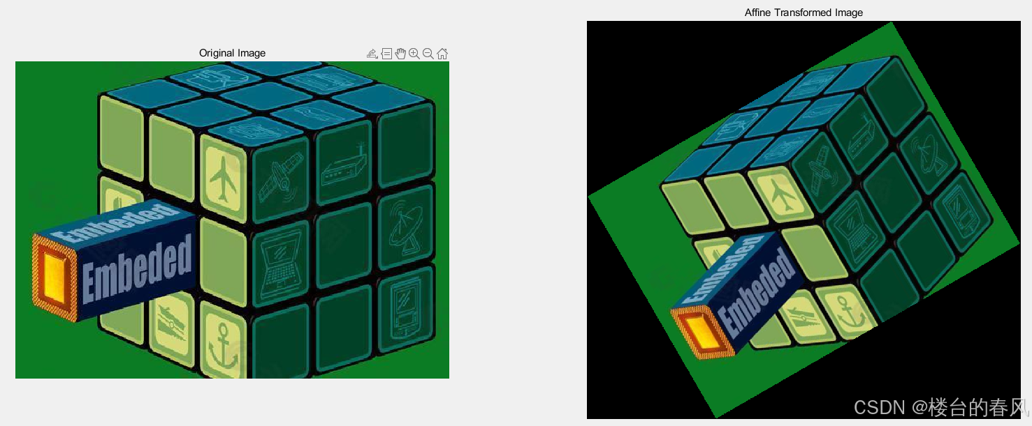
2. 仿射变换
• 对图像应用一个仿射变换,包括旋转30度和缩放1.5倍,显示变换后的图像。
matlab
c
% 读取图像
	img = imread('E:\Work\TestPic\embeded.jpg');

	% 定义仿射变换矩阵(旋转30度,缩放1.5倍)
	theta = 30; % 旋转角度
	scale = 1.5; % 缩放因子
	affineMatrix = [scale * cosd(theta), -scale * sind(theta), 0;
	                scale * sind(theta),  scale * cosd(theta), 0];

	% 创建affine2d对象(需要3x3矩阵)
	tform = affine2d([affineMatrix; 0 0 1]);

	% 应用仿射变换
	affineImg = imwarp(img, tform);

	% 显示结果
	figure;
	subplot(1, 2, 1);
	imshow(img);
	title('Original Image');
	subplot(1, 2, 2);
	imshow(affineImg);
	title('Affine Transformed Image');
运行结果:
3. 投影变换
• 对图像应用一个投影变换,模拟将图像从倾斜视角调整为正视图,显示变换后的图像。
matlab
c
% 读取图像
img = imread('peppers.png');
% 定义投影变换的控制点
% 原图中的四个角点坐标
originalPoints = [10, 10;
10, 200;
200, 10;
200, 200];
% 变换后的四个角点坐标
transformedPoints = [50, 50;
50, 250;
250, 50;
250, 250];
	% 计算投影变换矩阵
	tform = fitgeotrans(originalPoints, transformedPoints, 'projective');

	% 应用投影变换
	perspectiveImg = imwarp(img, tform, 'OutputView', imref2d([300, 300]));

	% 显示结果
	figure;
	subplot(1, 2, 1);
	imshow(img);
	title('Original Image');
	subplot(1, 2, 2);
	imshow(perspectiveImg);
	title('Perspective Transformed Image');
运行结果:

四、总结
通过今天的学习,已经掌握了图像几何变换的基本方法,包括平移、旋转、仿射变换和投影变换。这些变换在图像处理和计算机视觉中具有广泛的应用,例如图像对齐、拼接、透视校正等。通过实际练习,你可以进一步巩固这些知识,并尝试结合多种变换实现更复杂的图像处理任务。