Python 数据可视化全场景实现（一）

在学术研究与数据分析中，数据可视化是呈现研究成果、挖掘数据规律的重要手段。本文将通过 Python 的matplotlib和seaborn库，结合实际案例，详细介绍时间序列趋势、分组对比、数据分布、相关矩阵及多变量关系等多种场景下的数据可视化方法，并提供完整可复用代码。无论是论文撰写、报告展示，还是数据探索，都能找到实用的解决方案！大家喜欢就关注一下，代码可以直接运行！

一、可视化基础设置

在进行数据可视化之前，我们需要导入必要的库，并进行一些初始化设置，确保图表风格统一、美观。

import numpy as np
import pandas as pd
import matplotlib.pyplot as plt
import seaborn as sns
from matplotlib.gridspec import GridSpec

# 初始化设置
np.random.seed(42)
plt.style.use('seaborn-v0_8')  # 使用seaborn风格
sns.set_context("paper", font_scale=1.1)  # 设置适合论文的字体比例
palette = sns.color_palette("Set2")  # 定义颜色调色板

这里使用seaborn的风格和上下文设置，能够让图表在保持专业感的同时，具备良好的可读性。np.random.seed(42)确保随机数据的可重复性，方便调试和结果复现。

二、生成示例数据集

为了演示不同类型的可视化效果，我们生成五种常见的数据集：时间序列数据、分类数据、分布数据、相关矩阵数据和多维数据。

# 1. 时间序列数据
date_rng = pd.date_range(start='2020-01-01', end='2022-12-31', freq='M')
ts_data = np.cumsum(np.random.normal(0, 1.2, len(date_rng))) + 50

# 2. 分类数据
categories = ['A', 'B', 'C', 'D']
group1 = np.random.randint(20, 50, 4)
group2 = np.random.randint(15, 45, 4)

# 3. 分布数据
dist_data = [np.random.normal(loc=i, scale=1.2, size=100) for i in range(4)]
labels = ['Control', 'T1', 'T2', 'T3']

# 4. 相关矩阵
variables = ['X1', 'X2', 'X3', 'X4', 'X5']
corr_matrix = np.random.uniform(-0.8, 0.8, (5, 5))
np.fill_diagonal(corr_matrix, 1)

# 5. 多维数据
df = pd.DataFrame({
    'Var1': np.random.normal(0, 1.5, 200),
    'Var2': np.random.exponential(1, 200),
    'Category': np.random.choice(['Low', 'Medium', 'High'], 200)
})

这些数据集涵盖了从时间维度变化到变量间关系等多种分析场景，接下来我们将针对每种数据类型进行可视化。

三、多子图布局与可视化实现

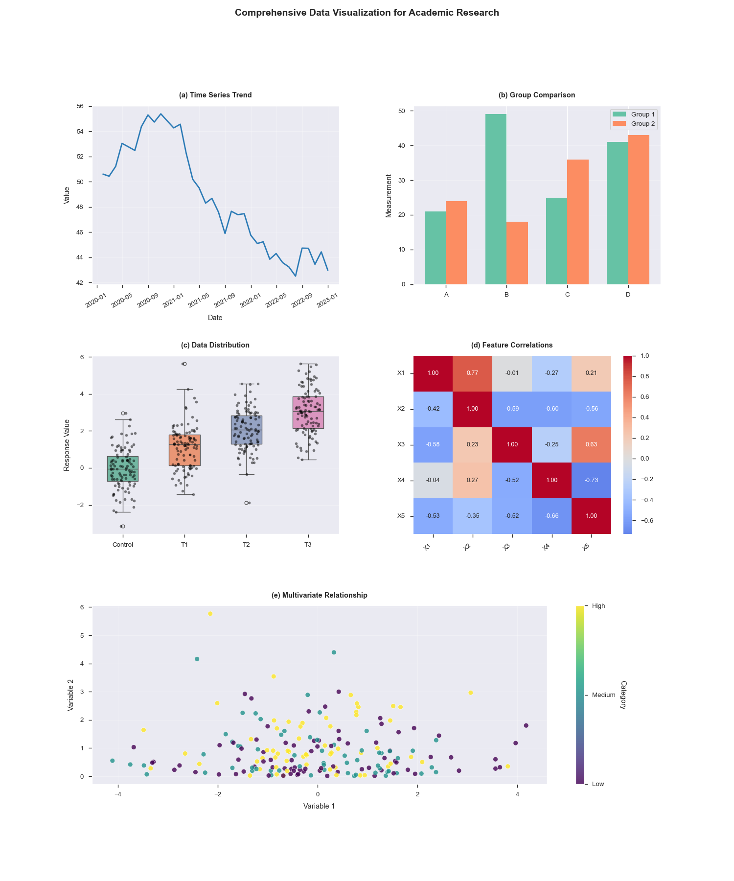
我们使用matplotlib的GridSpec来创建一个 3 行 2 列的子图布局，并在每个子图中展示不同类型的数据可视化效果。

3.1 子图 1：时间序列趋势

时间序列图常用于展示数据随时间的变化趋势，在学术研究中可用于分析实验指标、经济数据等的动态变化。

# 子图1：时间序列趋势
ax1 = fig.add_subplot(gs[0, 0])
ax1.plot(date_rng, ts_data, color='#2c7bb6', linewidth=2)
ax1.set_title('(a) Time Series Trend', pad=12, fontweight='semibold')
ax1.set_xlabel('Date', labelpad=8)
ax1.set_ylabel('Value', labelpad=8)
ax1.grid(alpha=0.3)
ax1.tick_params(axis='x', rotation=30)

通过plot函数绘制折线图，并设置颜色、线宽等参数增强可读性。tick_params调整横坐标标签的旋转角度，避免标签重叠。

3.2 子图 2：分组柱状图

柱状图适用于对比不同类别或组之间的数据差异，常用于实验结果对比、市场份额分析等场景。

# 子图2：分组柱状图
ax2 = fig.add_subplot(gs[0, 1])
x = np.arange(len(categories))
width = 0.35
rects1 = ax2.bar(x - width/2, group1, width, label='Group 1', color=palette[0])
rects2 = ax2.bar(x + width/2, group2, width, label='Group 2', color=palette[1])
ax2.set_title('(b) Group Comparison', pad=12, fontweight='semibold')
ax2.set_xticks(x)
ax2.set_xticklabels(categories)
ax2.legend(frameon=True, framealpha=0.9)
ax2.set_ylabel('Measurement', labelpad=8)
ax2.grid(axis='y', alpha=0.3)

使用bar函数绘制两组柱状图，并通过设置width和x坐标实现分组排列。legend函数添加图例，帮助区分不同组别。

3.3 子图 3：数据分布

箱线图和抖动图结合能够直观展示数据的分布特征、异常值及组间差异，常用于统计学分析和实验结果评估。

# 子图3：数据分布
ax3 = fig.add_subplot(gs[1, 0])
sns.boxplot(data=dist_data, palette='Set2', width=0.5, ax=ax3)
sns.stripplot(data=dist_data, color='black', alpha=0.5, jitter=0.2, size=4, ax=ax3)
ax3.set_title('(c) Data Distribution', pad=12, fontweight='semibold')
ax3.set_xticks(range(4))
ax3.set_xticklabels(labels)
ax3.set_ylabel('Response Value', labelpad=8)
ax3.grid(axis='y', alpha=0.3)

seaborn的boxplot和stripplot函数组合使用，箱线图展示数据的四分位数和异常值，抖动图则显示数据点的具体分布。

3.4 子图 4：相关矩阵

热力图是展示变量间相关性的有效工具，在数据分析和特征工程中常用于筛选关键变量。

# 子图4：相关矩阵
ax4 = fig.add_subplot(gs[1, 1])
sns.heatmap(corr_matrix, annot=True, cmap='coolwarm', center=0,
            fmt=".2f", annot_kws={"size":9}, ax=ax4)
ax4.set_title('(d) Feature Correlations', pad=12, fontweight='semibold')
ax4.set_xticks(np.arange(5)+0.5)
ax4.set_xticklabels(variables, rotation=45, ha='right')
ax4.set_yticks(np.arange(5)+0.5)
ax4.set_yticklabels(variables, rotation=0)

seaborn的heatmap函数自动生成热力图，并通过annot=True添加数值标注，cmap='coolwarm'使用冷暖色调区分正负相关性。

3.5 子图 5：多变量关系

散点图结合颜色编码能够展示多维数据中变量间的关系和类别分布，常用于探索性数据分析。

# 子图5：多变量关系
ax5 = fig.add_subplot(gs[2, :])  # 跨两列
sc = ax5.scatter(df['Var1'], df['Var2'], c=df['Category'].map({'Low':0, 'Medium':1, 'High':2}),
                cmap='viridis', alpha=0.8, s=50, edgecolor='w', linewidth=0.5)
ax5.set_title('(e) Multivariate Relationship', pad=12, fontweight='semibold')
ax5.set_xlabel('Variable 1', labelpad=8)
ax5.set_ylabel('Variable 2', labelpad=8)
cbar = fig.colorbar(sc, ax=ax5, ticks=[0, 1, 2])
cbar.set_ticklabels(['Low', 'Medium', 'High'])
cbar.set_label('Category', rotation=270, labelpad=15)
ax5.grid(alpha=0.3)

scatter函数绘制散点图，并通过c参数根据类别设置颜色。colorbar添加图例，清晰展示颜色与类别的对应关系。

四、全局调整与图表展示

最后，我们添加全局标题，并使用tight_layout优化子图布局，确保图表美观且信息完整。

# 全局调整
plt.suptitle("Comprehensive Data Visualization for Academic Research",
             y=0.99, fontsize=14, fontweight='bold')
plt.tight_layout()
plt.show(block=True)

五、可视化结果展示