机器学习：线性回归

线性回归
线性回归的实现

线性回归

线性回归的概念

线性回归是一种强大但有限制性的算法。当特征与整体的目标值呈现较强的线性关系时，可以使用线性回归进行拟合。但是需要说明，线性回归中，"线性"指的是参数是线性的，不是特征必须是线性的。例如：
y = w 1 x 1 + w 2 x 2 + b ( 1 ) y=w_1x_1+w_2x_2+b\quad \quad\quad\quad\quad\quad(1) y=w1x1+w2x2+b(1)
y = w 1 w 2 x 1 + w 3 x 2 + b ( 2 ) y=w_1w_2x_1+w_3x_2+b\quad \quad\quad\quad\quad(2) y=w1w2x1+w3x2+b(2)
y = w 1 x 2 + w 2 x 2 + b ( 3 ) y=w_1x^2+w_2x_2+b\quad\quad\quad\quad \quad\quad(3) y=w1x2+w2x2+b(3)

上述三个式子中，只有(2)是非线性的，而对于多项式拟合，也属于线性回归的一种。

损失函数的度量

损失函数指用来衡量预测值和真实值之间的偏差，在回归任务中，通常用均方误差(Mean Square Error,以下简称MSE)来衡量模型的预测能力。其计算方式如下：
M S E = ∑ i = 1 n ( y i − y i p ) 2 MSE=\sum_{i=1}^{n} (y_i-y^p_i)^2 MSE=i=1∑n(yi−yip)2

其中， y i y_i yi为实际值， y i p y^p_i yip为预测值。

优化函数

优化函数的目标是：找到让损失函数最小化的模型参数 。

主要有两种优化函数，即Adam和SGD

1.SGD随机梯度下降

SGD全称stochastic gradient descent，即随机梯度下降。其主要根据损失函数对各个参数的梯度来更新参数。随机梯度下降中的"随机"，指的是在对损失函数优化时，主要是沿着梯度的反方向进行优化，如果对整个训练集上的数据求解梯度，代价太大，此时一般会随机选取b个样本，使用这b个样本的损失来求解梯度。简化运算量。其主要学习以下两个内容：

1.梯度方向：参数应该向哪个方向能够减少损失

2.更新步长：学习率控制每次更新的幅度

2.Adam自适应学习率

Adam全称adaptive moment estimation，即自适应学习率。不仅学习梯度的方向，还学习每个参数的最佳学习率。主要学习以下三个内容：

1.梯度方向

2.梯度幅度(用于调整学习率)

3.每个参数独立的学习率

线性回归的实现

一元线性回归

使用sklearn实现

接下来，将从以下几个步骤进行实现：

①数据生成

②数据处理

③模型构建

④模型训练

⑤可视化

python 复制代码

# 使用sklearn实现LineRegression
import numpy as np
import matplotlib.pyplot as plt
from sklearn.model_selection import train_test_split
from sklearn.linear_model import LinearRegression
from sklearn.metrics import mean_squared_error as MSE
# 1.数据生成
np.random.seed(42)
X = np.linspace(0,10,100).reshape(-1,1)
y = 1.5*X.ravel()+2+np.random.normal(0,1,100)  # y=1.5x+2
# 2.数据处理
X_train,X_test,y_train,y_test = train_test_split(X,y,shuffle=True)
# 3.定义模型
model = LinearRegression()
# 4.模型训练
model.fit(X_train,y_train)
# 5.计算模型损失并可视化
X_train_pred = model.predict(X_train)
X_test_pred = model.predict(X_test)
train_mse = MSE(X_train_pred,y_train)
test_mse = MSE(X_test_pred,y_test)
print(f'目标函数为:y=1.5x+2,预测函数为:y={model.coef_[0]:.3f}x+{model.intercept_:.3f}')
print(f"测试集损失:{train_mse:.3f},训练集损失:{test_mse:.3f}")
plt.figure(figsize=(12,8))
pred_data = model.coef_[0]*X+model.intercept_
plt.scatter(X,y,label='Raw_Data')
plt.plot(X,pred_data,label='fit_line',color='red')
plt.legend()
plt.show()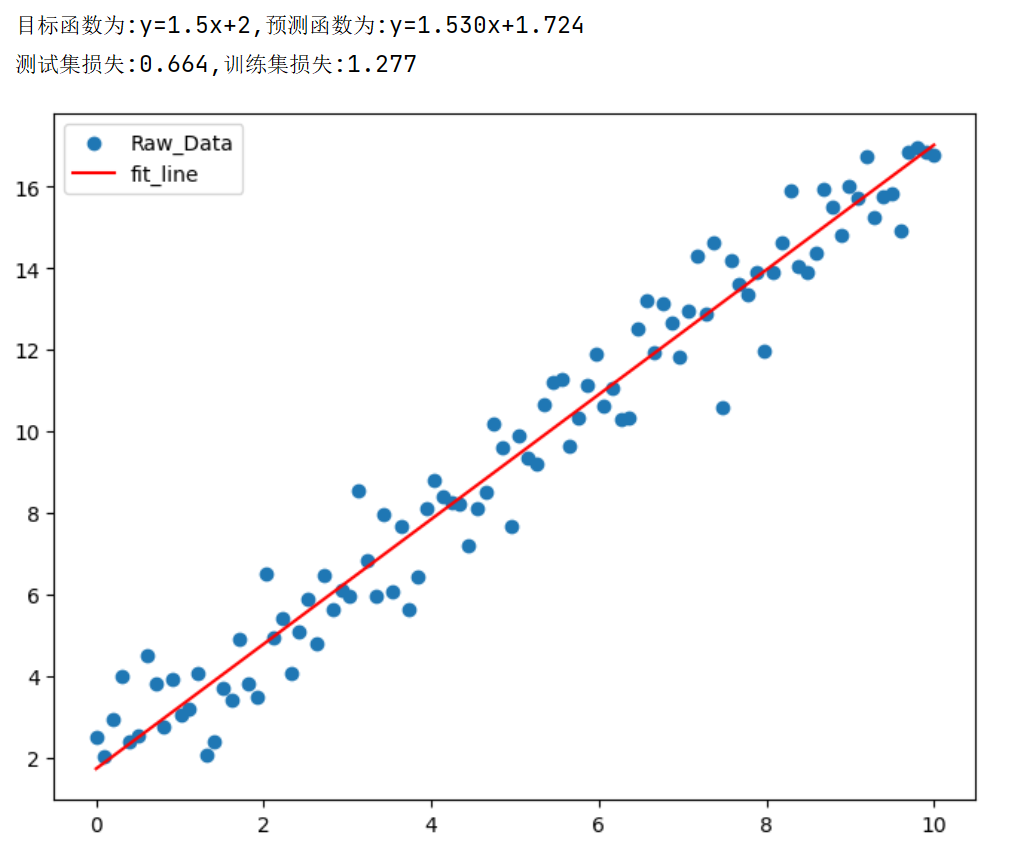

使用Pytorch实现

使用torch实现线性回归，从以下几个方面进行构建

①数据生成

②模型构建

③损失函数、优化器定义

④模型训练

⑥模型评估

⑦可视化

python 复制代码

# 使用torch实现LineRegression
import torch
import torch.nn as nn
import torch.optim as optim
import numpy as np
from sklearn.model_selection import train_test_split
np.random.seed(42)
# 1.生成数据
X = np.linspace(-3,3,100).reshape(-1,1)
y = 3*X+2+np.random.normal(0,1,100).reshape(-1,1)
# 2.转换为tensor数据类型
X_train,X_test,y_train,y_test = train_test_split(X,y,shuffle=True)
X_train_tensor = torch.from_numpy(X_train).float()
X_test_tensor = torch.from_numpy(X_test).float()
y_train_tensor = torch.from_numpy(y_train).float()
y_test_tensor = torch.from_numpy(y_test).float()
# 3.定义线性回归
class LineRegression(nn.Module):
    def __init__(self):
        super().__init__()
        self.linear = nn.Linear(1,1)
    def forward(self,x):
        output = self.linear(x)
        return output
# 4.定义损失函数,优化器等
model = LineRegression()
optimizer = optim.SGD(model.parameters(),lr=0.001) # 采用随机梯度下降
criterion = nn.MSELoss()  # 使用均方误差
losses = [] # 记录训练误差
# 5.训练模型
epochs = 1000
for epoch in range(epochs):
    outputs = model(X_train_tensor)
    loss = criterion(outputs,y_train_tensor)
    # 反向传播
    optimizer.zero_grad()  # 梯度清零
    loss.backward()        # 反向传播
    optimizer.step()
    losses.append(loss.item())
    if (epoch+1)%100==0:
        print(f'{epoch+1}/{epochs},loss:{loss:.3f}')
# 可视化衡量
plt.figure(figsize=(12,5))
# 绘制损失函数
plt.subplot(1,2,1)
plt.plot(losses)
plt.xlabel('epochs')
plt.ylabel('loss')
plt.title('Loss of Epochs')
# 绘制拟合图形
plt.subplot(1,2,2)
weight = model.linear.weight.item()
bias = model.linear.bias.item()
pred_data = weight*X+bias
print(X.shape)
print(y.shape)
plt.scatter(X,y,label='Raw_Point')
plt.plot(X,pred_data,label='Fit_line',color='red')
plt.show()
# 查看模型预测的参数
print(f'线性回归结果为:y={model.linear.weight.item():.3f}x+{model.linear.bias.item():.3f}')
print(f'原直线为:y=3x+2')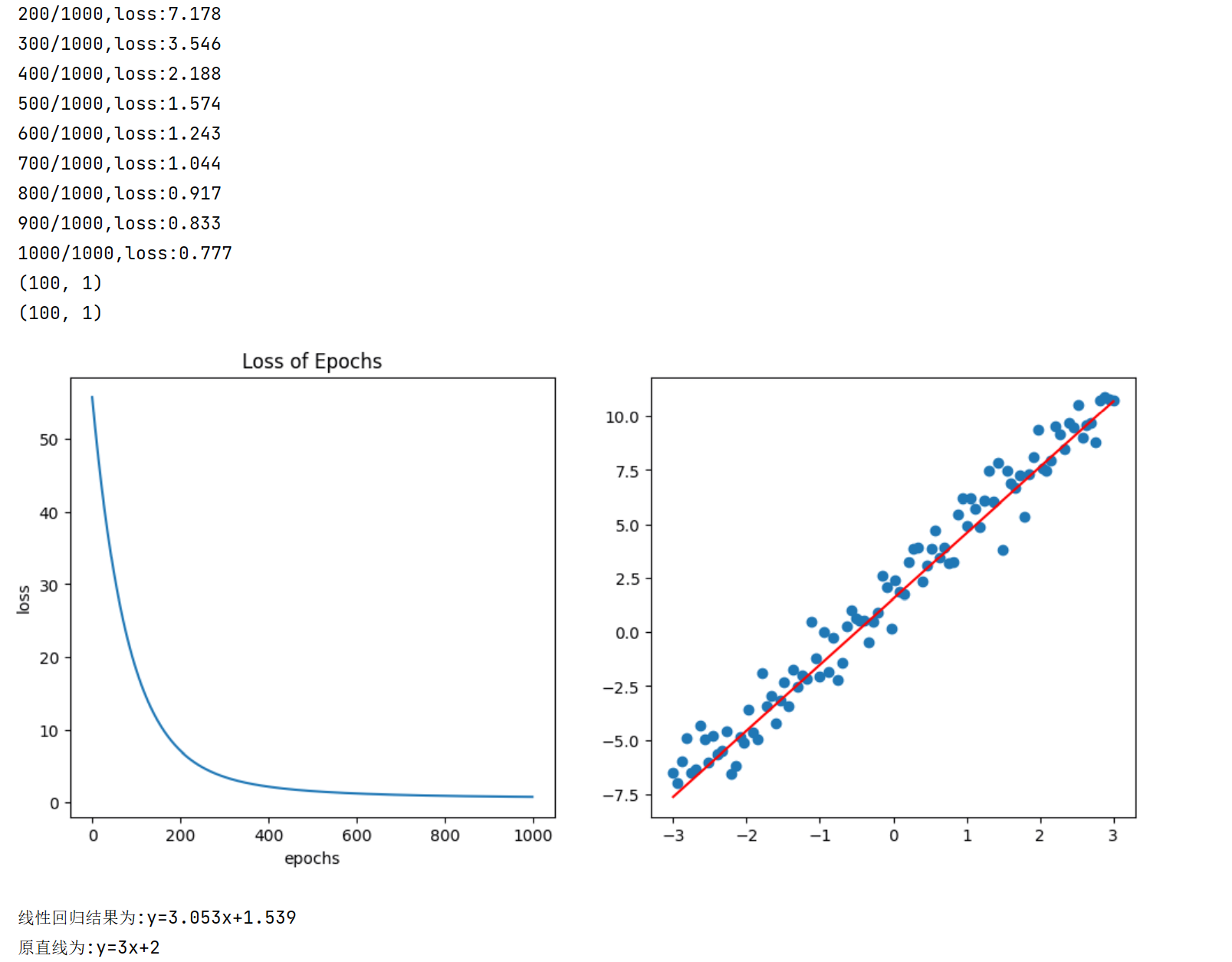

多项式回归

前面提过，多项式回归也属于线性回归。在这里，已三次函数为例，实现线性回归。

使用sklearn实现

python 复制代码

# 使用sklearn实现多项式回归
import numpy as np
import matplotlib.pyplot as plt
from sklearn.linear_model import LinearRegression
from sklearn.preprocessing import PolynomialFeatures
from sklearn.metrics import mean_squared_error as MSE
# np.random.seed(42)
# 1.生成数据
X = np.linspace(-3,3,100).reshape(-1,1)
y = 3*X.ravel()**3-2*X.ravel()**2+3*X.ravel()+1+np.random.normal(loc=0,scale=5,size=100)  # y=3x^3-2x^2+3x+1
# 2.特征工程
poly = PolynomialFeatures(degree=3)
X_features = poly.fit_transform(X,y)
# 3.模型构建与拟合
model = LinearRegression()
model.fit(X_features,y)
# 4.模型评估
pred = model.predict(X_features)
loss = MSE(pred,y)
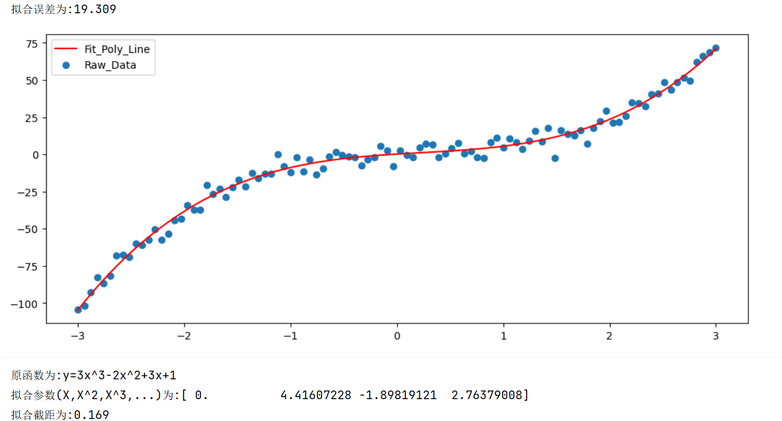
print(f"拟合误差为:{loss:.3f}")
# 5.可视化
plt.figure(figsize=(12,5))
plt.plot(X,pred,label='Fit_Poly_Line',color='red')
plt.scatter(X,y,label='Raw_Data')
plt.legend()
plt.show()
# 参数
print(f'原函数为:y=3x^3-2x^2+3x+1')
print(f'拟合参数(X,X^2,X^3,...)为:{model.coef_}')
print(f'拟合截距为:{model.intercept_:.3f}')

输出结果如下：

使用pytorch实现

使用pytorch更加灵活，能够调整参数以及训练轮次等信息。例如调整超参数degree可以拟合不同的次数

python 复制代码

# 使用torch实现线性回归
import torch
import torch.nn as nn
import torch.optim as optim
import numpy as np
np.random.seed(42)
# 1.生成数据
X = np.linspace(-3,3,100).reshape(-1,1)
y = 3*X.ravel()**3-2*X.ravel()**2+3*X.ravel()+1+np.random.normal(0,5,100)  # y=3x^3-2x^2+3x+1
# 2.转换为tensor类型
X_tensor = torch.from_numpy(X).float().view(-1,1)
y_tensor = torch.from_numpy(y).float().view(-1,1)
# 3.定义模型
class PolyRegression(nn.Module):
    def __init__(self,degree):
        super().__init__()
        self.linear = nn.Linear(degree,1)
    def forward(self,X):
        poly_features = torch.cat([X**i for i in range(1,self.linear.in_features+1)],dim=1)
        return self.linear(poly_features)
# 4.损失函数、优化器定义
degree = 3
model = PolyRegression(degree=degree)
criterion = nn.MSELoss()
optimizer = optim.Adam(model.parameters(),lr=0.01)
losses = []
# 5.模型训练
epochs = 1000
for epoch in range(epochs):
    # 前向传播
    outputs = model(X_tensor)
    # 计算损失
    loss = criterion(outputs,y_tensor)
    # 反向传播优化
    optimizer.zero_grad()
    loss.backward()
    optimizer.step()
    losses.append(loss.item())
    if (epoch+1)%100==0:
        print(f'{epoch+1}/{epochs},loss={loss:.3f}')
# 6.可视化
with torch.no_grad():
    predictions = model(X_tensor)
plt.figure(figsize=(12,5))
plt.subplot(1,2,1)
plt.plot(losses)
plt.title('Loss of Epochs')
plt.xlabel('Epochs')
plt.ylabel('Loss')
plt.subplot(1,2,2)
plt.scatter(X_tensor,y_tensor,label='Raw_data',color='black')
plt.plot(X_tensor,predictions,label='Fit_Poly_line',color='red')
plt.xlabel('X')
plt.ylabel('y')
plt.title('Scatter & Fit Line')
plt.legend()
plt.show()
# 7.参数输出
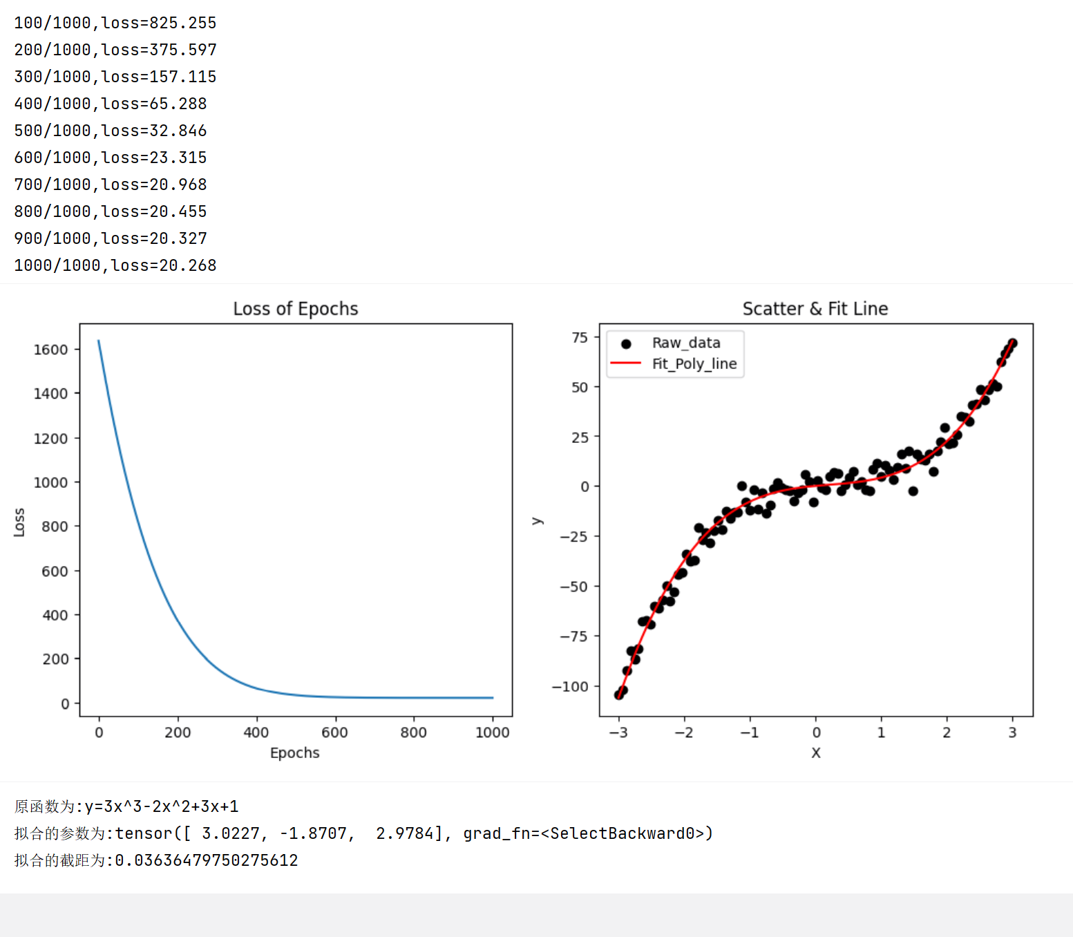
print(f'原函数为:y=3x^3-2x^2+3x+1')
print(f'拟合的参数为:{model.linear.weight[0]}')
print(f'拟合的截距为:{model.linear.bias.item()}')