小杰深度学习（five）——正则化、神经网络的过拟合解决方案

1. 正则化

正则化是通过在损失函数中添加正则化项 来控制模型复杂度、防止过拟合 的技术。机器学习中，复杂模型易过拟合（训练表现好、新数据泛化差），正则化通过约束参数抑制模型复杂度，常见正则化类型有 L1 和 L2 正则化。

损失函数的公式为：

1.当加上L1正则化后，损失函数变成：

2.当加上L2正则化后，损失函数变成：

1.1 为什么加入正则化可以解决过拟合？

加入正则化后，损失函数需同时最小化原损失（如 MSE）和正则化项 。以 L1/L2 为例，正则化项迫使参数 w 尽可能小，参数 w 小和解决过拟合的关系：

过拟合本质：模型因参数过多或数值过大而复杂，过度捕捉训练数据噪声。
参数越小 = 模型越简单：小参数限制模型对细节的拟合能力，降低复杂度，抑制过拟合（如削弱噪声特征的权重影响）。

总结：，正则化通过 "惩罚大参数 " 压缩模型表达能力，使其从 "记忆训练数据 " 转向 "学习通用规律"，从而提升泛化性。

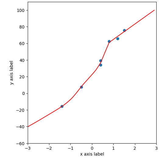
举个例子如下图曲线拟合散点：

1.2 正则化的基本思想

正则化的核心思想是在损失函数中引入与模型复杂度相关的额外项（如参数的 L1/L2 范数），通过调整正则化参数λ控制其权重，以惩罚模型复杂度，进而避免过拟合。

1.3 为什么只在W添加惩罚？

参数 b 是偏置项，仅控制拟合曲线沿 y 轴平移，不改变曲线形状。而正则化的目标是通过惩罚参数复杂度使曲线平滑，故对 b 施加正则化无实际意义。

1.4 L1正则化和L2正则化

以包含两个参数 w 1、w 2 的模型为例，左图为 L1 正则化 （约束区域为菱形），右图为 L2 正则化（约束区域为圆形），二者通过不同几何形状限制参数空间，实现复杂度惩罚。

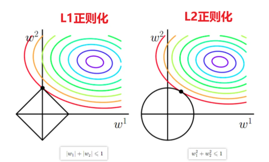
其中，L1正则化的约束条件为：

L2正则化的约束条件为：

以双参数 w 1,w 2 为例（彩色圈为损失等高线，中心损失最小）：

L1 正则化 （黑色菱形约束）：最优解易落在坐标轴上（如 w1=0），使参数稀疏（部分为 0），同时满足损失最小化与正则约束。
L2 正则化（黑色圆形约束）：最优解落在圆周与等高线切点，参数平滑缩小（非稀疏），损失函数常写为 Loss总=Loss原损失+1/22λw**2（含系数 1/2便于反向传播求导计算）。

2. 基本原理

2.1 散点输入

本实验中提供了一些散点，其分布如下图所示：

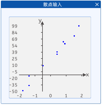
现在我们需要根据这些散点来拟合一条线，使我们可以根据这条线来预测新的散点的坐标。

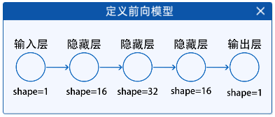
2.2 定义前向模型

定义前向模型，定义一个具有三个隐藏层的网络，来拟合这一条线。

2.3 定义损失函数和优化器

由于是拟合线问题，所以本实验选择的是MSE（均方误差损失函数）。

定义好损失函数后，就需要定义反向传播所需要的超参数了，需要对学习率和优化器以及正则化率进行选择，优化器这里选择的是Adam。正则化率默认选择的是0.001，不同的正则化率会对模型有较大的影响，如下图所示。

2.4 开始迭代

通过"开始迭代"组件，设置模型的训练次数。

2.5 显示频率设置

为了能够更好的观察迭代过程中的现象，可以通过"显示频率设置"组件来设置每隔多少次显示一次当前的拟合状态。

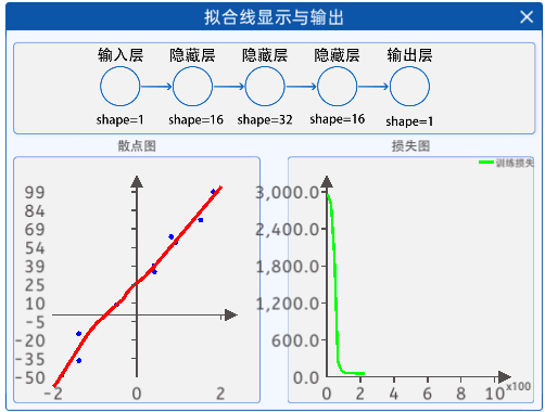
2.6 拟合线显示与输出

通过"拟合线显示与输出"组件，就可以观察到迭代过程中曲线的拟合状态了。

代码：

python 复制代码

import numpy as np
import torch
import torch.nn as nn
import matplotlib.pyplot as plt
#确保初始化的值都一样
seed=42
torch.manual_seed(seed)

# 1.创造数据，数据集
points = np.array([[-0.5, 7.7], [1.2, 65.8], [0.4, 39.2], [-1.4, -15.7],
                   [1.5, 75.6], [0.4, 34.0], [0.8, 62.3]])
# 分离特征和标签
x_train = points[:, 0]
y_train = points[:, 1]

# 2.定义前向模型
class Model(nn.Module):
    #定义初始化
    def __init__(self):
        super(Model,self).__init__()
        self.layer1=nn.Linear(1,16)
        self.layer2=nn.Linear(16,32)
        self.layer3=nn.Linear(32,16)
        self.layer4=nn.Linear(16,1)
    #前向过程
    def forward(self,x):
        #线性层后都跟着激活函数，实现非线性化
        x=torch.relu(self.layer1(x))
        x=torch.relu(self.layer2(x))
        x=torch.relu(self.layer3(x))
        # 最后一层是拟合回归不用激活
        x=self.layer4(x)
        return x

model=Model()

# 3.定义损失函数和优化器
#定义学习率
lr=0.05
#定义损失函数，这里是回归问题用mse
cri=torch.nn.MSELoss()
#定义优化器
#在梯度中添加正则化系数 weight_decay
optimizer=torch.optim.Adam(model.parameters(),lr=lr,weight_decay=0.2)

#7.画图
fig,(ax1,ax2) =plt.subplots(1,2,figsize=(12,6))
epoch_list=[]
loss_list=[]
# 4.开始迭代
epoches=1000
for epoch in range(1,epoches+1):
    #数据转化为tensor
    x_train_tensor=torch.tensor(x_train,dtype=torch.float32).unsqueeze(1)
    y_train_tensor=torch.tensor(y_train,dtype=torch.float32)
    #数据输入模型前向传播
    pre_result=model(x_train_tensor)
    #计算损失
    loss=cri(pre_result.squeeze(1),y_train_tensor)
    loss_list.append(loss.detach().numpy())
    epoch_list.append(epoch)
    #优化更新
    #梯度清零
    optimizer.zero_grad()
    #反向传播
    loss.backward()
    #参数更新
    optimizer.step()
    # 5.显示频率设置
    if epoch==1 or epoch%20==0:
        print(f"epoch:{epoch},loss:{loss}")
        # 6.绘图
        ax1.cla()
        ax1.scatter(x_train,y_train)
        x_range=torch.tensor(np.linspace(-2,2,100),dtype=torch.float32)
        y_range=model(x_range.unsqueeze(1))
        ax1.plot(x_range.detach().numpy(),y_range.detach().numpy().squeeze(1))
        ax2.cla()
        ax2.plot(epoch_list,loss_list)
        plt.pause(1)
plt.show()

2.神经网络的过拟合解决方案

1. 过拟合解决方案

1.1 神经网络的欠拟合解决方案

欠拟合出现的原因通常是数据量不足 、模型过于简单等因素导致的，那么可以通过适当的增加样本数据集 或增加神经网络隐藏层的层数来使神经网络复杂一点来解决欠拟合的问题。

1.2 神经网络的过拟合解决方案

过拟合出现的原因通常是模型过于复杂 或者数据量太少 ，导致过度学习训练模型中的细节和噪声。

在这里介绍两种过拟合的解决方案。

1.2.1 正则化

L1 和 L2 正则化，其核心是通过向损失函数添加正则化项惩罚模型参数大小，抑制过拟合。

1.2.2 Dropout

Dropout 是神经网络训练中通过随机 "丢弃 " 部分神经元输出（置为 0）的正则化技术，可降低模型对特定神经元的依赖，减少复杂度，增强泛化能力以抑制过拟合。

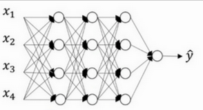
以某层含 4 个神经元的神经网络为例，来说明 dropout，如下图所示

若网络过拟合，可对各隐藏层应用 Dropout（参数 0.5）：该层每个节点以 50% 概率被随机置为 0（即类似执行"删除操作"），被置 0 的节点暂不参与前后层连接计算，以此降低模型复杂度，抑制过拟合。

如图所示）。

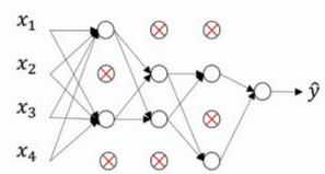
假设某隐藏层输出为 [0.7, 0.2, 0.9, 0.5]，应用 dropout（参数 0.5）后，部分神经元以 50% 概率被随机置 0，如变为 [0.7, 0, 0.9, 0]。此过程通过减少神经元间复杂依赖，降低模型复杂度，进而抑制过拟合。

1.2.2.1 Inverted Dropout(反向丢弃法)

训练时按 Dropout 概率随机舍弃神经元，对保留神经元的输出按比例缩放；测试时保留所有神经元。将权重按训练概率缩放，此方法称为反向丢弃法（Inverted Dropout）

python 复制代码

import torch
X=np.array([0.7,0.8,0.9,0.5])
# 在训练时
drop_prob=0.5
keep_prob = 1 - drop_prob   # keep_prob = 1-p即为保留率
mask = (torch.rand(X.shape) < keep_prob).float()
Y = mask * X / keep_prob
print(Y)
# 在测试时
# x

1.2.2.2 Dropout为什么能够解决过拟合：

（1）抑制过拟合 ：标准神经网络易依赖特定神经元导致过拟合，Dropout 通过随机丢弃神经元，迫使网络学习对神经元变化鲁棒的特征，降低对训练数据的过拟合。

（2）等效模型平均：训练时随机丢弃神经元相当于训练多个子网络，测试时保留全连接结构，预测结果等效于对各子网络输出取平均，通过 "综合抵消" 减轻过拟合。

代码展示：

python 复制代码

import numpy as np
import torch
import torch.nn as nn
import torch.optim as optim
import matplotlib.pyplot as plt

# 1.散点输入
class1_points = np.array(
    [[-0.7, 0.7], [3.9, 1.5], [1.7, 2.2], [1.9, -2.4], [0.9, 1.4], [4.2, 0.9], [1.7, 0.7], [0.2, -0.2], [3.1, -0.4],
     [-0.2, -0.9], [1.7, 0.2], [-0.6, -3.9], [-1.8, -4.0], [0.7, 3.8], [-0.7, -3.3], [0.8, 1.8], [-0.5, 1.5],
     [-0.6, -3.6], [-3.1, -3.0], [2.1, -2.5], [-2.5, -3.4], [-2.6, -0.8], [-0.2, 0.9], [-3.0, 3.3], [-0.7, 0.2],
     [0.3, 3.0], [0.6, 1.9], [-4.0, 2.4], [1.9, -2.2], [1.0, 0.3], [-0.9, -0.7], [-3.7, 0.6], [-2.7, -1.5], [0.9, -0.3],
     [0.8, -0.2], [-0.4, -4.4], [-0.3, 0.8], [4.1, 1.0], [-2.5, -3.5], [-0.8, 0.3], [0.6, 0.6], [2.6, -1.0], [1.8, 0.4],
     [1.5, -1.0], [3.2, 1.1], [3.3, -2.5], [-3.8, 2.5], [3.1, -0.9], [3.4, -1.1], [0.3, 0.8], [-0.1, 2.9], [-2.8, 1.9],
     [2.8, -3.3], [-1.0, 3.1], [-0.8, -0.6], [-2.5, -1.5], [0.3, 0.2], [-1.0, -2.9], [0.7, 0.2], [-0.5, 0.9],
     [-0.8, 0.7], [4.1, 0.5], [2.8, 2.3], [-3.9, 0.1], [2.2, -1.4], [-0.7, -3.5], [1.0, 1.2], [-0.7, -4.0], [1.3, 0.6],
     [-0.1, 3.3], [0.0, -0.3], [1.8, -3.0], [0.6, 0.0], [3.6, -2.8], [-3.9, -0.9], [-4.3, -0.9], [0.1, -0.8],
     [-1.6, -2.7], [-1.8, -3.3], [1.7, -3.5], [3.6, -3.1], [-2.4, 2.5], [-1.0, 1.8], [3.9, 2.5], [-3.9, -1.3],
     [3.4, 1.6], [-0.1, -0.6], [-3.7, -1.3], [-0.3, 3.4], [-3.7, -1.7], [4.0, 1.1], [3.4, 0.2], [0.1, -1.6],
     [-1.2, -0.5], [2.4, 1.7], [-4.4, -0.5], [-0.2, -3.6], [-0.8, 0.4], [-1.5, -2.2], [3.9, 2.5], [4.4, 1.4],
     [-3.5, -1.1], [-0.7, 1.5], [-3.0, -2.6], [0.2, -3.5], [0.0, 1.2], [-4.3, 0.1], [-1.8, 2.8], [1.1, -2.5],
     [0.2, 4.3], [-3.9, 2.2], [1.0, 1.6], [4.5, 0.2], [3.9, -1.6], [-0.4, -0.5], [0.3, -0.4], [-3.2, 1.7], [2.0, 4.1],
     [2.5, 2.2], [-1.1, -0.3], [-3.7, -1.9], [1.5, -1.1], [-2.1, -1.9], [-0.1, 4.5], [3.8, -0.3], [-0.9, -3.8],
     [-2.9, -1.6], [1.0, -1.2], [0.7, 0.0], [-0.8, 3.3], [-2.8, 3.1], [0.4, -3.2], [4.6, 1.0], [2.5, 3.1], [4.2, 0.8],
     [3.6, 1.8], [1.4, -3.0], [-0.4, -1.4], [-4.1, 1.1], [1.1, -0.2], [-2.9, -0.0], [-3.5, 1.3], [-1.4, 0.0],
     [-3.7, 2.2], [-2.9, 2.8], [1.7, 0.4], [-0.8, -0.6], [2.9, 1.1], [-2.3, 3.1], [-2.9, -2.0], [-2.7, -0.4],
     [2.6, -2.4], [-1.7, -2.8], [1.2, 3.1], [3.8, 1.3], [0.1, 1.9], [-0.5, -1.0], [0.0, -0.5], [3.9, -0.7],
     [-3.7, -2.5], [-3.1, 2.7], [-0.9, -1.0], [-0.7, -0.8], [-0.4, -0.1], [1.5, 1.0], [-2.6, 1.9], [-0.8, 1.7],
     [0.8, 1.8], [2.0, 3.6], [3.2, 1.4], [2.3, 1.4], [4.9, 0.5], [2.2, 1.8], [-1.4, -2.7], [3.1, 1.1], [-1.0, 3.8],
     [-0.4, -1.1], [3.3, 1.1], [2.2, -3.9], [1.0, 1.2], [2.6, 3.2], [-0.6, -3.0], [-1.9, -2.8], [1.2, -1.2],
     [-0.4, -2.7], [1.1, -4.3], [0.3, -0.8], [-1.0, -0.4], [-1.1, -0.2], [0.1, 1.2], [0.9, 0.6], [-2.7, 1.6],
     [1.0, -0.7], [0.3, -4.2], [-2.1, 3.2], [3.4, -1.2], [2.5, -4.0], [1.0, -0.8], [1.0, -0.9], [0.1, -0.6]])
class2_points = np.array(
    [[-3.0, -3.8], [4.4, 2.5], [2.6, 4.1], [3.7, -2.7], [-3.7, -2.9], [5.3, 0.3], [3.9, 2.9], [-2.7, -4.5], [5.4, 0.2],
     [3.0, 4.8], [-4.2, -1.3], [-2.1, -5.4], [-3.2, -4.6], [0.7, 4.5], [-1.4, -5.7], [0.5, 5.9], [-2.1, 4.0],
     [-0.1, -5.1], [-3.4, -4.7], [3.3, -4.7], [-2.7, -4.1], [-4.5, -2.0], [4.3, 2.9], [-3.6, 4.0], [-0.5, 5.5],
     [0.2, 5.2], [5.3, -0.9], [-4.5, 3.6], [3.4, -2.8], [-3.4, -3.7], [1.6, -5.5], [-5.9, -0.1], [-4.8, -2.5],
     [-5.5, 0.3], [1.6, 4.4], [-0.9, -5.3], [-1.0, 5.4], [4.9, 0.8], [-3.1, -4.0], [2.3, 4.7], [4.0, -1.6], [4.9, -1.5],
     [4.2, -2.5], [-3.5, 3.7], [4.7, 0.5], [5.3, -2.6], [-5.0, 2.4], [5.5, -1.2], [5.6, -1.3], [3.3, -4.3], [-1.3, 4.4],
     [-4.1, 3.6], [3.3, -4.5], [-2.3, 5.2], [2.6, 4.6], [-4.4, -1.6], [4.7, -2.0], [-1.7, -4.9], [-5.1, -2.4],
     [4.5, 3.2], [-3.9, -3.4], [6.0, -0.4], [3.5, 4.3], [-4.9, -0.6], [3.3, -3.2], [-0.3, -4.8], [-1.6, -4.7],
     [-1.4, -4.6], [-3.1, 3.8], [-1.4, 4.9], [1.8, -4.5], [2.2, -5.5], [3.1, -3.4], [4.7, -2.8], [-5.3, -0.4],
     [-6.0, -0.1], [1.4, -4.5], [-3.1, -4.3], [-1.8, -5.7], [1.7, -5.6], [4.5, -3.7], [-2.6, 4.3], [-3.4, 3.4],
     [4.7, 3.1], [-5.2, -2.8], [5.4, 1.2], [-5.4, 1.2], [-4.9, -1.3], [-1.3, 5.6], [-4.1, -2.6], [5.0, 1.0], [5.2, 1.2],
     [2.4, -4.9], [-3.2, 3.8], [3.3, 3.4], [-5.5, -0.8], [0.6, -5.0], [1.2, 5.4], [-3.4, -3.3], [4.6, 2.8], [5.2, 1.7],
     [-4.4, -0.9], [-5.0, -1.3], [-3.1, -3.6], [-0.7, -4.5], [5.9, -0.9], [-5.1, -0.5], [-2.6, 5.2], [1.4, -4.8],
     [-0.7, 5.6], [-5.3, 2.1], [4.9, 2.6], [5.3, 0.9], [5.1, -1.2], [2.7, -4.4], [-2.0, -5.6], [-4.9, 3.2], [2.8, 5.3],
     [2.6, 3.9], [-0.0, 5.7], [-5.7, -1.8], [-1.1, -4.7], [-2.4, -3.8], [-1.1, 5.6], [5.3, -1.5], [-0.4, -5.8],
     [-4.5, -1.6], [-4.4, -3.7], [-4.3, 2.4], [0.1, 4.8], [-3.0, 3.8], [0.3, -5.8], [5.6, 0.5], [4.1, 3.6], [5.0, 1.5],
     [5.7, 1.5], [3.2, -4.1], [-1.7, -5.6], [-5.3, 0.9], [4.3, 3.0], [-5.4, 0.3], [-5.0, 0.8], [2.7, 5.1], [-5.0, 2.2],
     [-4.0, 3.0], [-4.4, -3.9], [-3.5, -3.9], [5.3, 1.5], [-4.2, 4.2], [-3.9, -4.0], [-4.7, -0.1], [3.7, -4.7],
     [-3.0, -4.7], [2.7, 4.4], [4.3, 2.0], [-3.6, -4.5], [5.5, 0.9], [-4.7, -2.8], [5.5, -2.2], [-5.1, -2.6],
     [-3.6, 3.1], [-3.2, -4.0], [-4.8, 1.3], [-5.5, -1.6], [4.1, -1.6], [-4.2, 3.6], [5.6, -1.4], [4.9, -3.3],
     [1.7, 4.9], [5.3, 2.5], [3.8, 2.8], [5.8, 0.7], [3.9, 2.6], [-2.1, -4.8], [5.2, 2.5], [-2.0, 4.3], [2.8, -4.1],
     [5.6, 0.8], [2.2, -5.2], [-1.1, 5.5], [4.2, 3.8], [-1.8, -5.2], [-3.4, -3.6], [3.7, -3.6], [-0.5, -4.8],
     [1.9, -5.6], [-1.1, 5.4], [2.3, 4.7], [0.0, -5.4], [2.1, -5.6], [4.8, -0.3], [-4.7, 2.9], [-3.8, 3.9], [0.9, -5.5],
     [-2.3, 3.6], [5.3, -2.5], [3.7, -4.6], [-5.0, 2.4], [0.0, -5.7], [0.2, -5.9]])

# 合并两类点
points = np.concatenate((class1_points, class2_points), axis=0)
print(points)
# 标签0 表示类别1 ，标签1 表示类别2
labels1 = np.zeros(len(class1_points))
labels2 = np.ones(len(class2_points))
labels = np.concatenate((labels1, labels2))
# 2.定义前向模型
class ModelClass(nn.Module):
    def __init__(self):
        super(ModelClass, self).__init__()
        self.layer1 = nn.Linear(2, 8)
        self.layer2 = nn.Linear(8, 32)
        self.layer3 = nn.Linear(32, 32)
        self.layer4 = nn.Linear(32, 2)
        self.dropout1 = nn.Dropout(p=0.1)
        self.dropout2 = nn.Dropout(p=0.1)
        self.dropout3 = nn.Dropout(p=0.1)

    def forward(self, x):
        x = torch.relu(self.layer1(x))
        x = self.dropout1(x)
        x = torch.relu(self.layer2(x))
        x = self.dropout2(x)
        x = torch.relu(self.layer3(x))
        x = self.dropout3(x)
        # 二分类这里使用softmax加交叉熵
        x = torch.softmax(self.layer4(x), dim=1)
        return x


model = ModelClass()

# 3.定义损失函数和优化器
lr = 0.001
# 定义交叉熵损失函数
cri = nn.CrossEntropyLoss()
# 定义优化器
optimizer = optim.Adam(model.parameters(), lr=lr,weight_decay=0.01)

# 7.画图使用数据
x_min, x_max = points[:, 0].min() - 1, points[:, 0].max() + 1
y_min, y_max = points[:, 1].min() - 1, points[:, 1].max() + 1
step_size = 0.1
# 创建网格
xx, yy = np.meshgrid(np.arange(x_min, x_max, step_size),
                     np.arange(y_min, y_max, step_size))
grid_points = np.c_[xx.ravel(), yy.ravel()]
print(grid_points)
# 7.创建三维图形和右侧的二维子图
fig = plt.figure(figsize=(12, 8))
ax1_3d = fig.add_subplot(121, projection='3d')
ax2_2d = fig.add_subplot(122)

# 4.开始迭代
epoches = 500
batch_size = 8
for epoch in range(1, epoches + 1):
    # 进入训练模式
    model.train()
    # 按照batch_size进行迭代
    for batch_start in range(0, len(points), batch_size):
        batch_inputs = torch.tensor(points[batch_start:batch_start + batch_size, :], dtype=torch.float32)
        batch_labels = torch.tensor(labels[batch_start:batch_start + batch_size], dtype=torch.long)
        # 前向传播
        outputs = model(batch_inputs)
        # 计算loss
        loss = cri(outputs, batch_labels)
        #添加正则化项

        # 反向传播和优化
        optimizer.zero_grad()
        loss.backward()
        optimizer.step()

    # 进入验证模式
    model.eval()
    # 5.显示频率设置
    fre_display = 20
    # 显示与输出
    if epoch % fre_display == 0 or epoch == 1:
        # 使用训练好的模型预测网格点的标签
        # 转化为tensor
        grid_points_tensor = torch.tensor(grid_points, dtype=torch.float32)
        # 模型预测
        pre_result = model(grid_points_tensor)
        # 取出第一类的概率值
        pre_prob_one_class = pre_result[:, 0].reshape(xx.shape).detach().numpy()
        # 画ax1_3d图
        ax1_3d.cla()
        ax1_3d.scatter(class1_points[:, 0], class1_points[:, 1], np.ones_like(class1_points[:, 0]), c='blue',
                       label='class 1')
        ax1_3d.scatter(class2_points[:, 0], class2_points[:, 1], np.zeros_like(class2_points[:, 0]), c='red',
                       label='class 2')
        ax1_3d.legend()
        # 绘制三维表面图
        ax1_3d.plot_surface(xx, yy, pre_prob_one_class, alpha=0.5)
        ax1_3d.contour(xx, yy, pre_prob_one_class, levels=[0.5], cmap='jet')
        ax1_3d.set_xlabel('feature 1')
        ax1_3d.set_ylabel('feature 2')
        ax1_3d.set_zlabel('label')
        ax1_3d.set_title('hyperplane')

        # 绘制2d图
        ax2_2d.cla()
        ax2_2d.scatter(class1_points[:, 0], class1_points[:, 1], c='blue', label='Class 1')
        ax2_2d.scatter(class2_points[:, 0], class2_points[:, 1], c='red', label='Class 2')
        ax2_2d.contour(xx, yy, pre_prob_one_class, levels=[0.5], colors='black')
        plt.pause(1)
plt.show()