文章目录
- 深入解析MoE架构:大模型高效训练的核心技术
-
- 引言:大模型训练的效率困境
- 一、MoE架构的基本概念与历史演进
-
- [1.1 什么是混合专家(MoE)架构?](#1.1 什么是混合专家(MoE)架构?)
- [1.2 MoE的历史发展脉络](#1.2 MoE的历史发展脉络)
- 二、MoE架构的深入技术解析
-
- [2.1 核心组件与工作流程](#2.1 核心组件与工作流程)
- [2.2 负载均衡机制:MoE的关键挑战与解决方案](#2.2 负载均衡机制:MoE的关键挑战与解决方案)
- [2.3 容量因子与溢出处理](#2.3 容量因子与溢出处理)
- 三、MoE在现代大模型中的应用实践
-
- [3.1 GPT-4的MoE实现特点](#3.1 GPT-4的MoE实现特点)
- [3.2 DeepSeek的MoE优化策略](#3.2 DeepSeek的MoE优化策略)
- 四、MoE的训练策略与优化技巧
-
- [4.1 两阶段训练策略](#4.1 两阶段训练策略)
- [4.2 专家专业化引导](#4.2 专家专业化引导)
- 五、MoE的部署优化与推理加速
-
- [5.1 动态批处理与专家调度](#5.1 动态批处理与专家调度)
- [5.2 量化与压缩策略](#5.2 量化与压缩策略)
- 六、MoE的未来发展方向与挑战
-
- [6.1 技术挑战与解决方案](#6.1 技术挑战与解决方案)
- [6.2 未来研究方向](#6.2 未来研究方向)
- 七、实践指南:构建自己的MoE模型
-
- [7.1 快速开始示例](#7.1 快速开始示例)
- [7.2 性能调优建议](#7.2 性能调优建议)
- 结论
深入解析MoE架构:大模型高效训练的核心技术
引言:大模型训练的效率困境
在人工智能快速发展的今天,大型语言模型的参数规模已从数亿增长到数万亿。2023年,GPT-4的参数数量据估计达到1.8万亿,而谷歌的PaLM模型更是达到了惊人的5400亿参数。这种规模的增长带来了前所未有的性能提升,但同时也带来了巨大的计算挑战。
传统的密集模型架构面临着一个基本矛盾:模型规模与计算效率之间的权衡。当我们将模型参数增加10倍时,训练所需的计算资源通常会增加数十倍,推理延迟也会显著增加。这种指数级的增长使得大模型的训练和部署成本变得极其昂贵。
正是为了解决这一核心矛盾,混合专家(Mixture of Experts,MoE)架构应运而生。本文将深入探讨MoE架构的技术原理、实现方式、应用场景以及未来发展方向,为您揭示这一支撑现代大模型高效训练的核心技术。
一、MoE架构的基本概念与历史演进
1.1 什么是混合专家(MoE)架构?
混合专家模型是一种稀疏激活 的神经网络架构,其核心思想是将一个大型网络分解为多个"专家"子网络,但每次前向传播只激活其中的一小部分专家。这种设计允许模型在参数量巨大的同时,保持相对较低的计算成本。
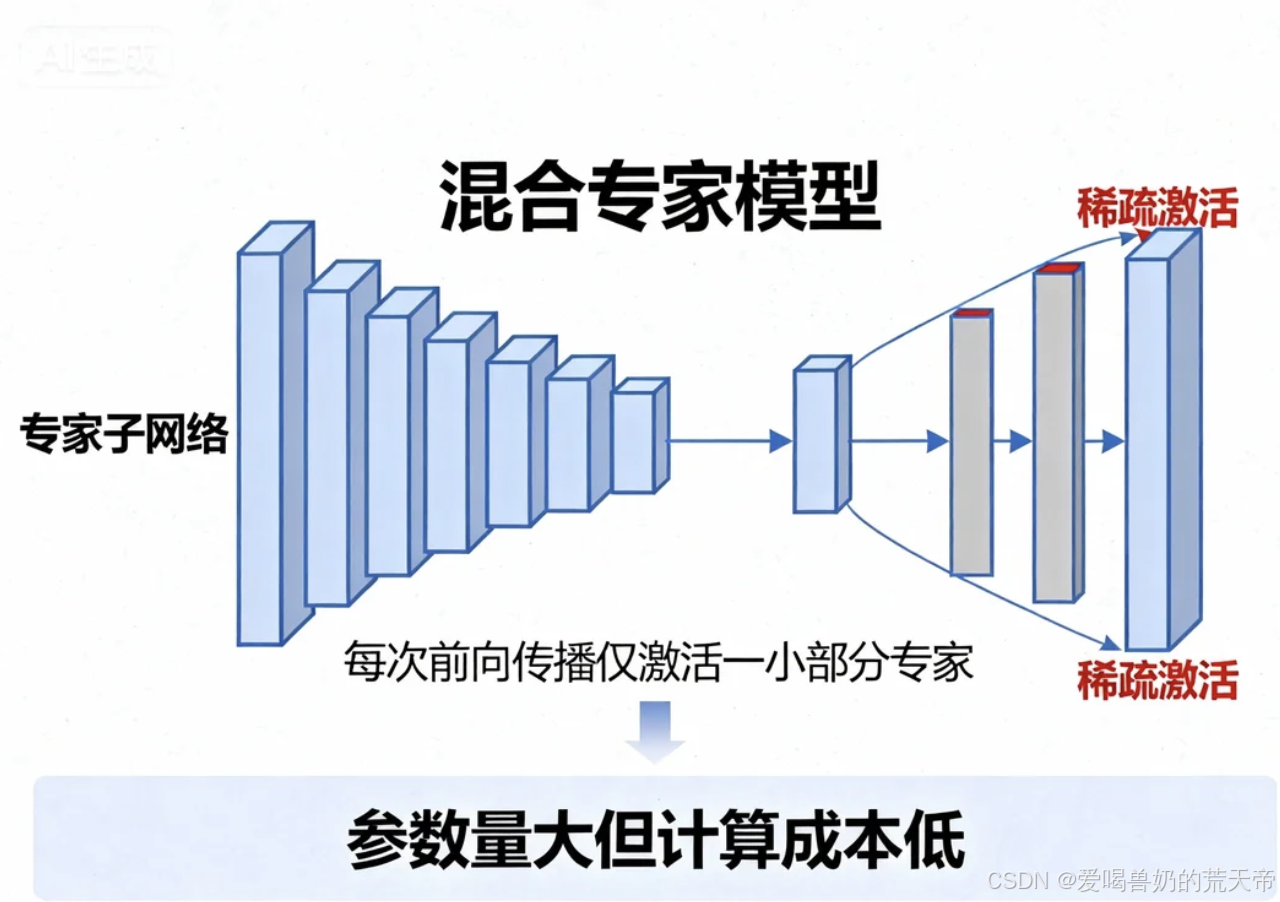
通俗理解:想象一个大型医院有100位各领域的专家医生,但每位病人只需要根据病情选择2-3位最相关的专家进行会诊。MoE就是这种"按需激活"的思想在神经网络中的体现。
1.2 MoE的历史发展脉络
MoE并非全新概念,其发展经历了几个关键阶段:
- 1991年:MoE概念首次由Jacobs等人提出,最初用于解决分类任务
- 2017年:Google Brain团队将MoE应用于大规模语言模型,推出Sparsely-Gated MoE
- 2020年:GShard(Google)将MoE扩展到分布式训练,实现6000亿参数模型
- 2021年:Switch Transformer(Google)简化MoE架构,实现万亿参数模型
- 2022-2024年:MoE成为大模型标配,GPT-4、Mixtral-8x7B、DeepSeek等均采用此架构
二、MoE架构的深入技术解析
2.1 核心组件与工作流程
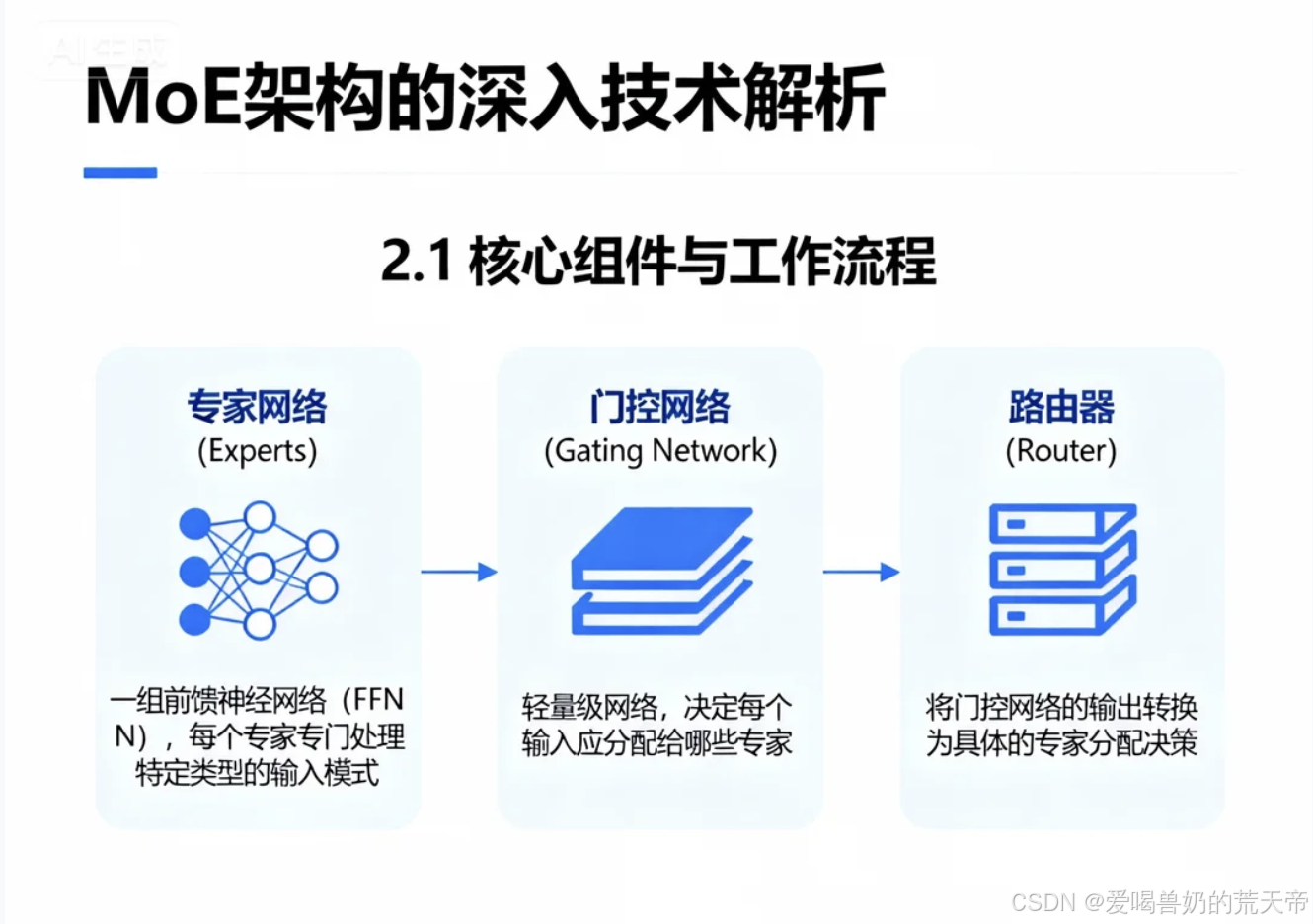
一个标准的MoE层包含三个核心组件:
- 专家网络(Experts):一组前馈神经网络(FFN),每个专家专门处理特定类型的输入模式
- 门控网络(Gating Network):轻量级网络,决定每个输入应分配给哪些专家
- 路由器(Router):将门控网络的输出转换为具体的专家分配决策
python
import torch
import torch.nn as nn
import torch.nn.functional as F

class Expert(nn.Module):
    """单个专家网络,通常是一个前馈神经网络"""
    def __init__(self, input_dim, hidden_dim, output_dim):
        super().__init__()
        self.fc1 = nn.Linear(input_dim, hidden_dim)
        self.fc2 = nn.Linear(hidden_dim, output_dim)
        self.dropout = nn.Dropout(0.1)

    def forward(self, x):
        x = self.fc1(x)
        x = F.gelu(x)  # 使用GELU激活函数
        x = self.dropout(x)
        x = self.fc2(x)
        return x


class SparseMoELayer(nn.Module):
    """稀疏MoE层实现"""
    def __init__(self, input_dim, output_dim, num_experts=8, capacity_factor=1.0, top_k=2):
        super().__init__()
        self.input_dim = input_dim
        self.output_dim = output_dim
        self.num_experts = num_experts
        self.capacity_factor = capacity_factor
        self.top_k = top_k  # 每个输入激活的专家数量

        # 创建专家池
        self.experts = nn.ModuleList([
            Expert(input_dim, 4 * input_dim, output_dim)
            for _ in range(num_experts)
        ])

        # 门控网络
        self.gate = nn.Linear(input_dim, num_experts)

    def forward(self, x):
        """
        前向传播过程
        x: [batch_size, seq_len, input_dim]
        返回: [batch_size, seq_len, output_dim]
        """
        batch_size, seq_len, _ = x.shape
        x_flat = x.reshape(-1, self.input_dim)  # 展平处理

        # 计算门控分数
        gate_logits = self.gate(x_flat)  # [batch_size*seq_len, num_experts]

        # 选择top_k专家
        top_k_vals, top_k_indices = torch.topk(
            gate_logits,
            k=self.top_k,
            dim=-1
        )

        # 计算门控权重(softmax over selected experts)
        top_k_weights = F.softmax(top_k_vals, dim=-1)

        # 初始化输出
        final_output = torch.zeros_like(x_flat)

        # 稀疏计算:只激活被选中的专家
        for expert_id in range(self.num_experts):
            # 找出需要当前专家处理的样本
            expert_mask = (top_k_indices == expert_id).any(dim=-1)

            if expert_mask.any():
                # 获取需要当前专家处理的输入
                expert_input = x_flat[expert_mask]

                # 计算专家输出
                expert_output = self.experts[expert_id](expert_input)

                # 获取对应的门控权重
                # 对于每个样本,找到当前专家在top_k中的位置
                sample_indices = torch.where(expert_mask)[0]
                weights_for_expert = torch.zeros(len(sample_indices), device=x.device)

                for i, sample_idx in enumerate(sample_indices):
                    # 找到该样本中当前专家的位置
                    expert_pos = (top_k_indices[sample_idx] == expert_id).nonzero(as_tuple=True)[0]
                    if len(expert_pos) > 0:
                        weights_for_expert[i] = top_k_weights[sample_idx, expert_pos[0]]

                # 加权求和
                final_output[expert_mask] += expert_output * weights_for_expert.unsqueeze(1)

        # 恢复原始形状
        return final_output.reshape(batch_size, seq_len, self.output_dim)
2.2 负载均衡机制:MoE的关键挑战与解决方案
负载不均衡是MoE架构面临的核心挑战之一。如果没有适当的控制机制,可能会出现"赢者通吃"现象------少数专家处理大部分输入,而多数专家很少被激活。
负载均衡的三种主要策略:
python
class LoadBalancingMoE(SparseMoELayer):
    """带有负载均衡的MoE层"""
    def __init__(self, input_dim, output_dim, num_experts=8,
                 top_k=2, balance_loss_weight=0.01):
        super().__init__(input_dim, output_dim, num_experts, top_k)
        self.balance_loss_weight = balance_loss_weight

    def compute_load_balancing_loss(self, gate_logits, top_k_indices):
        """
        计算负载均衡损失
        gate_logits: [batch_size*seq_len, num_experts]
        top_k_indices: [batch_size*seq_len, top_k]
        """
        batch_size_seq_len = gate_logits.shape[0]

        # 计算每个专家的选择概率(使用softmax)
        probs = F.softmax(gate_logits, dim=-1)  # [batch_size*seq_len, num_experts]

        # 计算每个专家的被选次数
        expert_mask = torch.zeros(
            (batch_size_seq_len, self.num_experts),
            device=gate_logits.device
        )

        # 创建one-hot编码的专家选择矩阵
        for k in range(self.top_k):
            expert_mask.scatter_(
                1,
                top_k_indices[:, k:k+1],
                1
            )

        # 计算负载均衡损失
        # 公式: L_balance = sum_i(sum_j P_ij * E_ij) / (N * E * sum_i P_i * E_i)
        P = probs.mean(dim=0)  # 平均选择概率 [num_experts]
        E = expert_mask.float().mean(dim=0)  # 实际选择频率 [num_experts]

        load_balance_loss = (P * E).sum() * self.num_experts

        return load_balance_loss

    def forward(self, x, return_balance_loss=False):
        # 标准前向传播
        batch_size, seq_len, _ = x.shape
        x_flat = x.reshape(-1, self.input_dim)

        gate_logits = self.gate(x_flat)
        top_k_vals, top_k_indices = torch.topk(gate_logits, k=self.top_k, dim=-1)
        top_k_weights = F.softmax(top_k_vals, dim=-1)

        # 计算负载均衡损失
        balance_loss = self.compute_load_balancing_loss(gate_logits, top_k_indices)

        # 稀疏计算(简化版)
        final_output = torch.zeros_like(x_flat)

        # 为简化示例,这里使用循环处理每个专家
        for expert_id in range(self.num_experts):
            expert_mask = (top_k_indices == expert_id).any(dim=-1)
            if expert_mask.any():
                expert_input = x_flat[expert_mask]
                expert_output = self.experts[expert_id](expert_input)

                # 获取对应权重
                sample_indices = torch.where(expert_mask)[0]
                weights = torch.zeros(len(sample_indices), device=x.device)

                for i, idx in enumerate(sample_indices):
                    expert_pos = (top_k_indices[idx] == expert_id).nonzero(as_tuple=True)[0]
                    if len(expert_pos) > 0:
                        weights[i] = top_k_weights[idx, expert_pos[0]]

                final_output[expert_mask] += expert_output * weights.unsqueeze(1)

        output = final_output.reshape(batch_size, seq_len, self.output_dim)

        if return_balance_loss:
            return output, balance_loss * self.balance_loss_weight

        return output
2.3 容量因子与溢出处理
在实际部署中,MoE层需要处理专家容量限制的问题。每个专家只能处理有限数量的token,超出部分需要特殊处理。
python
class MoEWithCapacity(SparseMoELayer):
    """带有容量控制的MoE层"""
    def __init__(self, input_dim, output_dim, num_experts=8,
                 top_k=2, capacity_factor=1.2):
        super().__init__(input_dim, output_dim, num_experts, top_k)
        self.capacity_factor = capacity_factor

    def forward(self, x):
        batch_size, seq_len, input_dim = x.shape
        num_tokens = batch_size * seq_len

        # 计算每个专家的容量
        expert_capacity = int(self.capacity_factor * num_tokens / self.num_experts)
        expert_capacity = max(expert_capacity, 4)  # 确保最小容量

        # 展平输入
        x_flat = x.reshape(-1, input_dim)

        # 门控计算
        gate_logits = self.gate(x_flat)
        top_k_vals, top_k_indices = torch.topk(gate_logits, k=self.top_k, dim=-1)
        top_k_weights = F.softmax(top_k_vals, dim=-1)

        # 创建调度矩阵
        final_output = torch.zeros_like(x_flat)

        # 处理每个专家
        for expert_id in range(self.num_experts):
            # 找到需要该专家的所有token
            token_indices = torch.where((top_k_indices == expert_id).any(dim=1))[0]

            if len(token_indices) == 0:
                continue

            # 如果超过容量,只处理前capacity个token
            if len(token_indices) > expert_capacity:
                # 根据门控分数排序,选择分数最高的capacity个token
                expert_gates = gate_logits[token_indices, expert_id]
                _, sorted_indices = torch.topk(expert_gates, k=expert_capacity)
                selected_tokens = token_indices[sorted_indices]

                # 标记溢出的token(可选:用其他专家处理或丢弃)
                overflow_tokens = token_indices[~torch.isin(token_indices, selected_tokens)]
                # 这里简单丢弃溢出token,实际应用中可能需要更复杂的处理
            else:
                selected_tokens = token_indices

            if len(selected_tokens) > 0:
                # 处理选中的token
                expert_input = x_flat[selected_tokens]
                expert_output = self.experts[expert_id](expert_input)

                # 应用权重
                for i, token_idx in enumerate(selected_tokens):
                    # 找到该token中当前专家的位置
                    pos = (top_k_indices[token_idx] == expert_id).nonzero(as_tuple=True)[0]
                    if len(pos) > 0:
                        weight = top_k_weights[token_idx, pos[0]]
                        final_output[token_idx] += expert_output[i] * weight

        return final_output.reshape(batch_size, seq_len, self.output_dim)
三、MoE在现代大模型中的应用实践
3.1 GPT-4的MoE实现特点
根据OpenAI公开的技术报告和相关信息,GPT-4的MoE实现具有以下特点:
- 分层MoE结构:在不同网络层使用不同配置的MoE
- 动态专家选择:根据输入内容动态调整激活的专家数量
- 专业化训练:通过预训练策略使专家形成不同领域的专业知识

python
class GPT4StyleMoE(nn.Module):
    """模拟GPT-4风格的MoE实现"""
    def __init__(self, config):
        super().__init__()
        self.config = config
        self.num_layers = config.num_layers

        # 创建不同配置的MoE层
        self.moe_layers = nn.ModuleList()
        for layer_idx in range(self.num_layers):
            # 在不同层使用不同数量的专家
            if layer_idx < config.num_layers // 3:
                num_experts = 4  # 底层使用较少专家
            elif layer_idx < 2 * config.num_layers // 3:
                num_experts = 8  # 中层
            else:
                num_experts = 16  # 高层使用更多专家

            moe_layer = LoadBalancingMoE(
                input_dim=config.hidden_size,
                output_dim=config.hidden_size,
                num_experts=num_experts,
                top_k=config.moe_top_k,
                balance_loss_weight=config.balance_loss_weight
            )
            self.moe_layers.append(moe_layer)

    def forward(self, hidden_states):
        """前向传播"""
        moe_losses = []

        for i, moe_layer in enumerate(self.moe_layers):
            # 残差连接
            residual = hidden_states

            # 通过MoE层
            if self.training:
                hidden_states, balance_loss = moe_layer(
                    hidden_states,
                    return_balance_loss=True
                )
                moe_losses.append(balance_loss)
            else:
                hidden_states = moe_layer(hidden_states)

            # 层归一化和残差连接
            hidden_states = F.layer_norm(
                hidden_states + residual,
                normalized_shape=(self.config.hidden_size,)
            )

        # 计算总的MoE损失
        total_moe_loss = torch.stack(moe_losses).mean() if moe_losses else None

        return hidden_states, total_moe_loss
3.2 DeepSeek的MoE优化策略
DeepSeek在MoE实现上进行了多项创新优化:
- 专家共享策略:在不同层之间共享部分专家参数
- 细粒度路由:在序列级别而非token级别进行专家选择
- 训练稳定性优化:特殊的初始化方法和梯度裁剪策略
python
class DeepSeekMoE(nn.Module):
    """DeepSeek风格的MoE实现"""
    def __init__(self, config):
        super().__init__()
        self.config = config

        # 共享专家池:所有层共享同一组专家
        self.shared_experts = nn.ModuleList([
            Expert(
                config.hidden_size,
                config.expert_hidden_size,
                config.hidden_size
            ) for _ in range(config.num_shared_experts)
        ])

        # 每层特定的门控网络
        self.layer_gates = nn.ModuleList([
            nn.Linear(config.hidden_size, config.num_shared_experts)
            for _ in range(config.num_layers)
        ])

        # 局部专家(每层独有的专家)
        self.local_experts = nn.ModuleList([
            nn.ModuleList([
                Expert(
                    config.hidden_size,
                    config.expert_hidden_size,
                    config.hidden_size
                ) for _ in range(config.num_local_experts)
            ]) for _ in range(config.num_layers)
        ])

        self.local_gates = nn.ModuleList([
            nn.Linear(config.hidden_size, config.num_local_experts)
            for _ in range(config.num_layers)
        ])

    def forward(self, hidden_states, layer_idx):
        """
        前向传播
        layer_idx: 当前层索引
        """
        batch_size, seq_len, hidden_dim = hidden_states.shape

        # 展平处理
        x_flat = hidden_states.reshape(-1, hidden_dim)

        # 共享专家计算
        shared_gate_logits = self.layer_gates[layer_idx](x_flat)
        shared_probs = F.softmax(shared_gate_logits, dim=-1)

        # 局部专家计算
        local_gate_logits = self.local_gates[layer_idx](x_flat)
        local_probs = F.softmax(local_gate_logits, dim=-1)

        # 合并专家输出
        output = torch.zeros_like(x_flat)

        # 处理共享专家
        top_k_shared = min(2, self.config.num_shared_experts)
        shared_top_k_vals, shared_top_k_indices = torch.topk(
            shared_probs, k=top_k_shared, dim=-1
        )
        shared_top_k_weights = F.softmax(shared_top_k_vals, dim=-1)

        for i in range(top_k_shared):
            expert_id = shared_top_k_indices[:, i]
            expert_weight = shared_top_k_weights[:, i]

            # 为每个样本选择对应的专家
            for batch_idx in range(x_flat.shape[0]):
                current_expert_id = expert_id[batch_idx].item()
                current_weight = expert_weight[batch_idx]

                expert_output = self.shared_experts[current_expert_id](
                    x_flat[batch_idx:batch_idx+1]
                )
                output[batch_idx] += expert_output.squeeze(0) * current_weight

        # 处理局部专家(类似方式)
        top_k_local = min(1, self.config.num_local_experts)
        local_top_k_vals, local_top_k_indices = torch.topk(
            local_probs, k=top_k_local, dim=-1
        )
        local_top_k_weights = F.softmax(local_top_k_vals, dim=-1)

        for i in range(top_k_local):
            expert_id = local_top_k_indices[:, i]
            expert_weight = local_top_k_weights[:, i]

            for batch_idx in range(x_flat.shape[0]):
                current_expert_id = expert_id[batch_idx].item()
                current_weight = expert_weight[batch_idx]

                expert_output = self.local_experts[layer_idx][current_expert_id](
                    x_flat[batch_idx:batch_idx+1]
                )
                output[batch_idx] += expert_output.squeeze(0) * current_weight

        return output.reshape(batch_size, seq_len, hidden_dim)
四、MoE的训练策略与优化技巧
4.1 两阶段训练策略
MoE模型通常采用两阶段训练策略:
python
class MoETrainingScheduler:
    """MoE训练调度器"""
    def __init__(self, total_steps, warmup_steps=1000):
        self.total_steps = total_steps
        self.warmup_steps = warmup_steps
        self.current_step = 0

    def get_training_phase(self):
        """获取当前训练阶段"""
        if self.current_step < self.warmup_steps:
            return "warmup"  # 热身阶段
        elif self.current_step < self.total_steps * 0.3:
            return "stage1"  # 第一阶段:基础能力训练
        else:
            return "stage2"  # 第二阶段:专家专业化训练

    def get_training_config(self, phase):
        """根据阶段返回训练配置"""
        configs = {
            "warmup": {
                "learning_rate": 1e-5,
                "balance_loss_weight": 0.0,  # 热身阶段不应用负载均衡损失
                "dropout_rate": 0.0,
                "gradient_clip": 1.0
            },
            "stage1": {
                "learning_rate": 3e-4,
                "balance_loss_weight": 0.01,
                "dropout_rate": 0.1,
                "gradient_clip": 0.5
            },
            "stage2": {
                "learning_rate": 1e-4,
                "balance_loss_weight": 0.02,  # 增加负载均衡约束
                "dropout_rate": 0.2,
                "gradient_clip": 0.2
            }
        }
        return configs.get(phase, configs["stage2"])

    def step(self):
        self.current_step += 1
4.2 专家专业化引导
为了促使不同专家形成专业化能力,可以采用以下策略:
python
class ExpertSpecializationTrainer:
    """专家专业化训练器"""
    def __init__(self, num_experts, specialization_dim=128):
        self.num_experts = num_experts
        self.specialization_dim = specialization_dim

        # 为每个专家创建一个专业化向量
        self.expert_specializations = nn.Parameter(
            torch.randn(num_experts, specialization_dim)
        )

        # 专业化目标:鼓励专家处理特定类型的输入
        self.specialization_loss_weight = 0.1

    def compute_specialization_loss(self, expert_outputs, expert_ids, input_features):
        """
        计算专业化损失
        expert_outputs: 专家输出列表
        expert_ids: 使用的专家ID
        input_features: 输入特征
        """
        loss = 0.0

        for expert_id in range(self.num_experts):
            # 找出该专家处理的样本
            mask = (expert_ids == expert_id)
            if mask.any():
                # 获取该专家处理的输入特征
                expert_inputs = input_features[mask]

                # 计算输入特征与专家专业化向量的相似度
                # 我们希望专家处理与其专业化方向相似的输入
                similarity = F.cosine_similarity(
                    expert_inputs[:, :self.specialization_dim],
                    self.expert_specializations[expert_id].unsqueeze(0),
                    dim=-1
                )

                # 专业化损失:鼓励相似度高
                loss += (1 - similarity.mean())

        return loss * self.specialization_loss_weight / self.num_experts
五、MoE的部署优化与推理加速
5.1 动态批处理与专家调度
在实际部署中,MoE模型的推理优化至关重要:
python
class MoEInferenceOptimizer:
    """MoE推理优化器"""
    def __init__(self, model, max_batch_size=32, use_cuda_graph=False):
        self.model = model
        self.max_batch_size = max_batch_size
        self.use_cuda_graph = use_cuda_graph

        # 缓存专家输出(针对重复计算)
        self.expert_cache = {}

    def optimize_inference(self, inputs):
        """
        优化推理过程
        inputs: 输入张量列表
        """
        # 动态批处理
        batched_inputs = self.dynamic_batching(inputs)

        # 专家调度优化
        optimized_outputs = []

        for batch in batched_inputs:
            # 预计算门控决策
            gate_decisions = self.precompute_gates(batch)

            # 优化专家调度
            expert_schedule = self.schedule_experts(gate_decisions)

            # 执行推理
            if self.use_cuda_graph and len(batch) == self.max_batch_size:
                output = self.cuda_graph_inference(batch, expert_schedule)
            else:
                output = self.standard_inference(batch, expert_schedule)

            optimized_outputs.append(output)

        return self.unbatch_outputs(optimized_outputs)

    def schedule_experts(self, gate_decisions):
        """优化专家调度,减少计算重叠"""
        # 按专家ID分组输入
        expert_groups = {}

        for token_idx, (expert_ids, weights) in enumerate(gate_decisions):
            for expert_id, weight in zip(expert_ids, weights):
                if expert_id not in expert_groups:
                    expert_groups[expert_id] = []
                expert_groups[expert_id].append((token_idx, weight))

        # 排序专家以减少内存跳转
        schedule = []
        for expert_id in sorted(expert_groups.keys()):
            schedule.append((expert_id, expert_groups[expert_id]))

        return schedule
5.2 量化与压缩策略
python
class MoEQuantizer:
    """MoE模型量化器"""
    def __init__(self, model, quantization_bits=8):
        self.model = model
        self.quantization_bits = quantization_bits

    def quantize_experts(self):
        """量化专家权重"""
        for name, module in self.model.named_modules():
            if isinstance(module, Expert):
                self.quantize_module(module)

    def quantize_module(self, module):
        """量化单个模块"""
        # 权重量化
        if hasattr(module, 'weight'):
            weight = module.weight.data
            quantized_weight = self.quantize_tensor(weight)
            module.weight.data = quantized_weight

        # 激活量化(动态范围)
        module.activation_precision = self.quantization_bits

    def quantize_tensor(self, tensor):
        """量化张量"""
        if self.quantization_bits == 8:
            # 8-bit量化
            scale = tensor.abs().max() / 127.0
            quantized = torch.clamp(torch.round(tensor / scale), -128, 127)
            return quantized * scale
        elif self.quantization_bits == 4:
            # 4-bit量化(更激进)
            # 这里使用简单的分块量化
            tensor_flat = tensor.flatten()
            num_blocks = (tensor_flat.shape[0] + 31) // 32

            quantized_blocks = []
            for i in range(num_blocks):
                block = tensor_flat[i*32:(i+1)*32]
                block_min, block_max = block.min(), block.max()
                scale = (block_max - block_min) / 15.0

                quantized_block = torch.clamp(
                    torch.round((block - block_min) / scale),
                    0, 15
                )
                quantized_blocks.append(quantized_block * scale + block_min)

            quantized = torch.cat(quantized_blocks)[:tensor_flat.shape[0]]
            return quantized.reshape(tensor.shape)

        return tensor
六、MoE的未来发展方向与挑战
6.1 技术挑战与解决方案
| 挑战 | 描述 | 当前解决方案 | 未来方向 |
|---|---|---|---|
| 负载不均衡 | 少数专家处理大部分输入 | 负载均衡损失函数 | 动态专家容量 |
| 通信开销 | 分布式训练中的专家通信 | 专家分组、分层MoE | 更智能的路由策略 |
| 训练不稳定 | MoE特有的梯度问题 | 梯度裁剪、特殊初始化 | 改进的优化算法 |
| 内存占用 | 专家参数存储 | 专家共享、参数复用 | 更高效的内存管理 |
6.2 未来研究方向
- 自适应MoE:根据输入复杂度动态调整专家数量
- 跨模态MoE:处理文本、图像、音频的多模态专家
- 联邦学习中的MoE:隐私保护下的分布式专家训练
- 神经架构搜索优化:自动发现最优MoE结构
七、实践指南:构建自己的MoE模型
7.1 快速开始示例
python
import torch
from torch import nn
import torch.nn.functional as F

class SimpleMoEModel(nn.Module):
    """简单的MoE模型示例"""
    def __init__(self, vocab_size=50000, hidden_size=768,
                 num_experts=8, num_layers=12):
        super().__init__()

        # 词嵌入层
        self.embedding = nn.Embedding(vocab_size, hidden_size)

        # MoE层
        self.moe_layers = nn.ModuleList([
            SparseMoELayer(
                input_dim=hidden_size,
                output_dim=hidden_size,
                num_experts=num_experts,
                top_k=2
            ) for _ in range(num_layers)
        ])

        # 输出层
        self.output_layer = nn.Linear(hidden_size, vocab_size)

        # 层归一化
        self.layer_norm = nn.LayerNorm(hidden_size)

    def forward(self, input_ids):
        # 嵌入层
        x = self.embedding(input_ids)

        # 通过MoE层
        for moe_layer in self.moe_layers:
            residual = x
            x = moe_layer(x)
            x = self.layer_norm(x + residual)

        # 输出层
        logits = self.output_layer(x)

        return logits

# 使用示例
model = SimpleMoEModel()
input_ids = torch.randint(0, 50000, (4, 128))  # batch_size=4, seq_len=128
logits = model(input_ids)
print(f"输出形状: {logits.shape}")  # 应该是 [4, 128, 50000]
7.2 性能调优建议
- 专家数量选择:从小规模开始(4-8个专家),逐步增加
- 容量因子设置:开始时设为1.2-1.5,根据溢出率调整
- 负载均衡权重:从0.01开始,观察专家利用率
- 批处理策略:使用动态批处理优化推理速度
结论
MoE架构作为大模型高效训练的核心技术,已经在GPT-4、DeepSeek等先进模型中证明了其价值。通过稀疏激活机制,MoE在保持模型容量的同时大幅降低了计算成本,为实现更大规模的模型提供了可行的技术路径。
然而,MoE技术仍处于快速发展阶段,面临负载均衡、训练稳定性、推理优化等诸多挑战。随着研究的深入和工程实践的积累,我们有理由相信MoE将在未来的人工智能发展中发挥更加重要的作用。
对于开发者和研究者来说,理解MoE的原理和实现细节,掌握其优化技巧,将有助于构建更高效、更强大的AI系统。本文提供的代码示例和实践建议,希望能为您在MoE领域的探索提供有价值的参考。