EM算法详解：解密“鸡生蛋“的机器学习困局

引言：当"先有鸡还是先有蛋"遇到机器学习

假设你有两枚外观相同的硬币，它们被设计成抛出正面的概率不同，但你既不知道每次用的是哪枚，也不知道它们各自的真实概率。可能是硬币A是70%，硬币B是30%；也可能是硬币A是80%，硬币B是20%------你对此完全一无所知。

现在，你进行了100次实验：

1. 每次实验，你随机拿起一枚硬币（但你不知道拿的是哪一枚）
2. 将这枚硬币抛掷10次，记录正反面结果
3. 重复这个过程

现在你只有100组抛掷结果。挑战来了：如何从这些数据中，**同时推断出两枚硬币各自的正面概率？**仔细分析这个问题，你会发现你同时面临两个"不知道"：

1. 不知道隐变量：对于每一次实验，你都不知道自己用的是硬币A还是硬币B
2. 不知道参数：你也不知道两枚硬币各自的正面概率是多少

这形成了经典的"鸡生蛋"困局：

• 要知道每次用的硬币，需要知道硬币的概率
• 要知道硬币的概率，又需要知道每次用的硬币
• 简单平均所有数据只会得到一个混合概率，无法揭示两枚硬币的真实情况。

EM算法通过"先猜后证"的迭代方式破解这个困局：

• 先猜：随机假设两枚硬币的概率，如硬币A=0.6，硬币B=0.5
• 分配：基于假设，评估每组数据来自各硬币的可能性
• 修正：根据可能性重新计算概率
• 重复：用新概率重新分配，再修正，直到结果稳定

这个看似循环的方法，实际上包含强大的自我修正能力。如果硬币A的真实概率更高，那么抛出较多正面的结果自然会更多被分配给它，从而在修正时提高它的概率估计。反之，硬币B则会得到更多反面数据，降低其概率估计。这形成了"分配强化估计，估计改进分配"的正向循环。即使从错误的初始猜测开始，经过多次迭代，两枚硬币的概率也会逐渐分开，最终逼近真实值。

EM算法揭示了一个深刻道理：面对双重未知，我们可以从任意起点开始，让数据引导我们逐步逼近真相。这不仅是机器学习的核心思想，也反映了人类认知世界的基本方式------通过不断的假设、验证和修正，在不确定性中寻找确定性。

一、EM算法手动推导：抛硬币例子详解

1.1 符号定义

• 两枚硬币：硬币A和硬币B
• 硬币A的正面概率：θA\theta_AθA（待估计）
• 硬币B的正面概率：θB\theta_BθB（待估计）
• 实验轮数：n=5n=5n=5轮
• 每轮抛掷次数：m=10m=10m=10次
• 第iii轮观测数据：xix_ixi 是10次抛掷的具体正反面序列
• 我们记 hih_ihi 为第iii轮观测中正面出现的次数，ti=10−hit_i = 10 - h_iti=10−hi 为反面次数
• 隐变量：zi∈{A,B}z_i \in \{A, B\}zi∈{A,B}，表示第iii轮选择的硬币

重要说明 ：由于每次抛掷是独立的，任何具有相同正面次数hhh的序列都具有相同的概率。具体来说，如果硬币正面概率为θ\thetaθ，那么产生一个具体序列（包含hhh次正面和ttt次反面）的概率为 θh(1−θ)t\theta^h (1-\theta)^tθh(1−θ)t。在比较不同硬币产生该序列的概率时，我们只需要关心hhh和ttt，因此可以用(hi,ti)(h_i, t_i)(hi,ti)来概括观测数据。

我们的观测数据为（正面次数和反面次数）：

轮数i	正面次数hih_ihi	反面次数tit_iti
1	5	5
2	9	1
3	8	2
4	1	9
5	1	9

为了直观理解，这里给出每轮可能的序列示例（注意：任何具有相同hih_ihi的序列概率相同，这里只是示例）：

• 第1轮（5正5反）：正正正正正反反反反反
• 第2轮（9正1反）：正正正正正正正正正反
• 第3轮（8正2反）：正正正正正正正正反反
• 第4轮（1正9反）：正反反反反反反反反反
• 第5轮（1正9反）：正反反反反反反反反反

1.2 一次完整的EM迭代

初始化

θA(0)=0.6,θB(0)=0.5 \theta_A^{(0)} = 0.6, \quad \theta_B^{(0)} = 0.5 θA(0)=0.6,θB(0)=0.5

E步：计算隐变量后验分布

对于每一轮iii，计算：
γiA(t)=P(zi=A∣xi,θ(t))=θA(t)hi(1−θA(t))10−hiθA(t)hi(1−θA(t))10−hi+θB(t)hi(1−θB(t))10−hi \gamma_{iA}^{(t)} = P(z_i=A|x_i,\theta^{(t)}) = \frac{\theta_A^{(t)h_i}(1-\theta_A^{(t)})^{10-h_i}}{\theta_A^{(t)h_i}(1-\theta_A^{(t)})^{10-h_i} + \theta_B^{(t)h_i}(1-\theta_B^{(t)})^{10-h_i}} γiA(t)=P(zi=A∣xi,θ(t))=θA(t)hi(1−θA(t))10−hi+θB(t)hi(1−θB(t))10−hiθA(t)hi(1−θA(t))10−hi

（假设先验P(zi=A)=P(zi=B)=0.5P(z_i=A)=P(z_i=B)=0.5P(zi=A)=P(zi=B)=0.5，分子分母同时乘以0.5后约去）

用向量化表示，记θA=θA(t)\theta_A = \theta_A^{(t)}θA=θA(t)，θB=θB(t)\theta_B = \theta_B^{(t)}θB=θB(t)：

轮数i	计算过程	γiA(t)\gamma_{iA}^{(t)}γiA(t)结果
1	0.65×0.450.65×0.45+0.510\frac{0.6^5 \times 0.4^5}{0.6^5 \times 0.4^5 + 0.5^{10}}0.65×0.45+0.5100.65×0.45	0.4487
2	0.69×0.410.69×0.41+0.510\frac{0.6^9 \times 0.4^1}{0.6^9 \times 0.4^1 + 0.5^{10}}0.69×0.41+0.5100.69×0.41	0.8053
3	0.68×0.420.68×0.42+0.510\frac{0.6^8 \times 0.4^2}{0.6^8 \times 0.4^2 + 0.5^{10}}0.68×0.42+0.5100.68×0.42	0.7334
4,5	0.61×0.490.61×0.49+0.510\frac{0.6^1 \times 0.4^9}{0.6^1 \times 0.4^9 + 0.5^{10}}0.61×0.49+0.5100.61×0.49	0.1386

同理，γiB(t)=1−γiA(t)\gamma_{iB}^{(t)} = 1 - \gamma_{iA}^{(t)}γiB(t)=1−γiA(t)。

M步：重新估计参数

最大化Q函数：
Q(θ∣θ(t))=∑i=15[γiA(t)log⁡(θAhi(1−θA)10−hi)+γiB(t)log⁡(θBhi(1−θB)10−hi)] Q(\theta|\theta^{(t)}) = \sum_{i=1}^5 \left[ \gamma_{iA}^{(t)} \log(\theta_A^{h_i}(1-\theta_A)^{10-h_i}) + \gamma_{iB}^{(t)} \log(\theta_B^{h_i}(1-\theta_B)^{10-h_i}) \right] Q(θ∣θ(t))=i=1∑5[γiA(t)log(θAhi(1−θA)10−hi)+γiB(t)log(θBhi(1−θB)10−hi)]

对θA\theta_AθA和θB\theta_BθB分别求导并令导数为0，得到闭式解：

θA(t+1)=∑i=15γiA(t)hi10∑i=15γiA(t) \theta_A^{(t+1)} = \frac{\sum_{i=1}^5 \gamma_{iA}^{(t)} h_i}{10 \sum_{i=1}^5 \gamma_{iA}^{(t)}} θA(t+1)=10∑i=15γiA(t)∑i=15γiA(t)hi

θB(t+1)=∑i=15γiB(t)hi10∑i=15γiB(t) \theta_B^{(t+1)} = \frac{\sum_{i=1}^5 \gamma_{iB}^{(t)} h_i}{10 \sum_{i=1}^5 \gamma_{iB}^{(t)}} θB(t+1)=10∑i=15γiB(t)∑i=15γiB(t)hi

代入数值计算：

θA(1)=0.4487×5+0.8053×9+0.7334×8+0.1386×1+0.1386×110×(0.4487+0.8053+0.7334+0.1386+0.1386)=0.6902 \theta_A^{(1)} = \frac{0.4487 \times 5 + 0.8053 \times 9 + 0.7334 \times 8 + 0.1386 \times 1 + 0.1386 \times 1}{10 \times (0.4487 + 0.8053 + 0.7334 + 0.1386 + 0.1386)} = 0.6902 θA(1)=10×(0.4487+0.8053+0.7334+0.1386+0.1386)0.4487×5+0.8053×9+0.7334×8+0.1386×1+0.1386×1=0.6902

θB(1)=0.5513×5+0.1947×9+0.2666×8+0.8614×1+0.8614×110×(0.5513+0.1947+0.2666+0.8614+0.8614)=0.3058 \theta_B^{(1)} = \frac{0.5513 \times 5 + 0.1947 \times 9 + 0.2666 \times 8 + 0.8614 \times 1 + 0.8614 \times 1}{10 \times (0.5513 + 0.1947 + 0.2666 + 0.8614 + 0.8614)} = 0.3058 θB(1)=10×(0.5513+0.1947+0.2666+0.8614+0.8614)0.5513×5+0.1947×9+0.2666×8+0.8614×1+0.8614×1=0.3058

1.3 迭代过程与收敛

迭代次数ttt	θA(t)\theta_A^{(t)}θA(t)	θB(t)\theta_B^{(t)}θB(t)
0	0.6000	0.5000
1	0.6902	0.3058
2	0.7758	0.1891
3	0.8316	0.1209
4	0.8567	0.0937
5	0.8662	0.0827
10	≈0.8687	≈0.0789

经过约10次迭代，参数基本收敛到：
θA≈0.87,θB≈0.08 \theta_A ≈ 0.87, \quad \theta_B ≈ 0.08 θA≈0.87,θB≈0.08

1.4 结果解释

• 算法成功区分出两枚硬币：一枚高概率（0.87），一枚低概率（0.08）
• 正面次数多的数据（第2、3轮）被分配给硬币A，正面次数少的数据（第4、5轮）被分配给硬币B
• 第1轮（5正5反）最难判断，后验概率接近0.5:0.5
• EM算法通过迭代逐步改进了参数估计，即使从错误的初始猜测开始

二、程序模拟

import warnings
from typing import List, Tuple, Dict

import matplotlib
import matplotlib.pyplot as plt
import numpy as np

matplotlib.rcParams['axes.unicode_minus'] = False
matplotlib.rcParams['font.family'] = 'Kaiti SC'
warnings.filterwarnings('ignore')

# 设置中文字体
plt.rcParams['font.sans-serif'] = ['SimHei']
plt.rcParams['axes.unicode_minus'] = False


# ==================== 第一部分：数据模拟 ====================

def simulate_coin_experiments(
        theta_A: float = 0.8,  # 硬币A的真实正面概率
        theta_B: float = 0.3,  # 硬币B的真实正面概率
        n_experiments: int = 20,  # 实验次数
        n_tosses: int = 20,  # 每次实验抛掷次数
        seed: int = 42  # 随机种子
) -> Tuple[List[int], List[str]]:
    """
    模拟硬币抛掷实验

    参数:
        theta_A: 硬币A的正面概率
        theta_B: 硬币B的正面概率
        n_experiments: 实验次数
        n_tosses: 每次实验抛掷次数
        seed: 随机种子

    返回:
        heads_counts: 每次实验的正面次数列表
        true_coins: 每次实验真实使用的硬币列表
    """
    np.random.seed(seed)

    heads_counts = []
    true_coins = []

    for _ in range(n_experiments):
        # 随机选择硬币（假设先验概率各为0.5）
        if np.random.random() < 0.5:
            true_coin = 'A'
            theta = theta_A
        else:
            true_coin = 'B'
            theta = theta_B

        # 进行n_tosses次抛掷
        tosses = np.random.random(n_tosses) < theta
        heads_count = int(np.sum(tosses))

        heads_counts.append(heads_count)
        true_coins.append(true_coin)

    return heads_counts, true_coins


# ==================== 第二部分：EM算法核心 ====================

def compute_posterior(
        heads_count: int,
        theta_A: float,
        theta_B: float,
        n_tosses: int = 20
) -> Tuple[float, float]:
    """
    计算单次实验的后验概率

    参数:
        heads_count: 正面次数
        theta_A: 硬币A的当前估计概率
        theta_B: 硬币B的当前估计概率
        n_tosses: 抛掷次数

    返回:
        gamma_A: 属于硬币A的概率
        gamma_B: 属于硬币B的概率
    """
    # 计算两种假设下的似然
    if theta_A > 0 and theta_A < 1:
        likelihood_A = (theta_A ** heads_count) * ((1 - theta_A) ** (n_tosses - heads_count))
    else:
        likelihood_A = 0

    if theta_B > 0 and theta_B < 1:
        likelihood_B = (theta_B ** heads_count) * ((1 - theta_B) ** (n_tosses - heads_count))
    else:
        likelihood_B = 0

    # 避免数值下溢
    if likelihood_A == 0 and likelihood_B == 0:
        likelihood_A = likelihood_B = 1e-10

    # 假设先验概率相等，计算后验概率
    total = likelihood_A + likelihood_B

    if total == 0:
        gamma_A = gamma_B = 0.5
    else:
        gamma_A = likelihood_A / total
        gamma_B = likelihood_B / total

    return gamma_A, gamma_B


def em_algorithm_for_coins(
        heads_counts: List[int],
        initial_theta_A: float = 0.6,
        initial_theta_B: float = 0.5,
        n_tosses: int = 20,
        max_iterations: int = 10,
        tolerance: float = 1e-6
) -> Dict:
    """
    EM算法估计硬币概率

    参数:
        heads_counts: 每次实验的正面次数列表
        initial_theta_A: 硬币A的初始估计
        initial_theta_B: 硬币B的初始估计
        n_tosses: 每次实验抛掷次数
        max_iterations: 最大迭代次数
        tolerance: 收敛阈值

    返回:
        result_dict: 包含所有结果的字典
    """
    n_experiments = len(heads_counts)

    # 初始化参数
    theta_A = initial_theta_A
    theta_B = initial_theta_B

    # 记录迭代历史
    theta_A_history = [theta_A]
    theta_B_history = [theta_B]

    for iteration in range(max_iterations):
        # ========== E步 ==========
        # 初始化统计量
        weighted_heads_A = 0.0
        weighted_heads_B = 0.0
        total_weight_A = 0.0
        total_weight_B = 0.0

        # 计算后验概率并累计统计量
        for h in heads_counts:
            gamma_A, gamma_B = compute_posterior(h, theta_A, theta_B, n_tosses)

            weighted_heads_A += gamma_A * h
            weighted_heads_B += gamma_B * h
            total_weight_A += gamma_A
            total_weight_B += gamma_B

        # ========== M步 ==========
        # 更新参数
        new_theta_A = weighted_heads_A / (total_weight_A * n_tosses) if total_weight_A > 0 else theta_A
        new_theta_B = weighted_heads_B / (total_weight_B * n_tosses) if total_weight_B > 0 else theta_B

        # 避免参数越界
        new_theta_A = max(0.001, min(0.999, new_theta_A))
        new_theta_B = max(0.001, min(0.999, new_theta_B))

        # 检查收敛
        delta_A = abs(new_theta_A - theta_A)
        delta_B = abs(new_theta_B - theta_B)

        # 更新参数
        theta_A = new_theta_A
        theta_B = new_theta_B

        # 记录历史
        theta_A_history.append(theta_A)
        theta_B_history.append(theta_B)

        # 打印当前迭代信息
        print(f"迭代 {iteration + 1}: θ_A = {theta_A:.4f}, θ_B = {theta_B:.4f}")

        # 检查收敛
        if max(delta_A, delta_B) < tolerance:
            print(f"在第{iteration + 1}次迭代后收敛")
            break

    return {
        'theta_A_history': theta_A_history,
        'theta_B_history': theta_B_history,
        'final_theta_A': theta_A,
        'final_theta_B': theta_B,
        'n_iterations': len(theta_A_history) - 1
    }


# ==================== 快速演示版本 ====================

def quick_demo():
    """快速演示版本"""
    print("EM算法快速演示")
    print("-" * 40)

    # 设置实验参数
    true_theta_A = 0.9
    true_theta_B = 0.7
    n_experiments = 20
    n_tosses = 30

    print(f"实验设置:")
    print(f"  - 总实验次数: {n_experiments}")
    print(f"  - 每次实验抛掷次数: {n_tosses}")
    print(f"  - 硬币A的真实正面概率: {true_theta_A:.2f}")
    print(f"  - 硬币B的真实正面概率: {true_theta_B:.2f}")
    print()

    # 1. 简单模拟数据
    np.random.seed(42)

    # 生成20个简单数据点
    heads_counts, true_coins = simulate_coin_experiments(
        theta_A=true_theta_A,
        theta_B=true_theta_B,
        n_experiments=n_experiments,
        n_tosses=n_tosses,
        seed=42
    )

    # 2. 运行EM算法
    print(f"每次实验的正面次数: {heads_counts}")
    print(f"\nEM算法迭代过程:")

    result = em_algorithm_for_coins(
        heads_counts=heads_counts,
        initial_theta_A=0.6,
        initial_theta_B=0.5,
        n_tosses=n_tosses,
        max_iterations=10
    )

    print(f"\n最终估计结果:")
    print(f"  θ_A (估计) = {result['final_theta_A']:.4f} (真实: {true_theta_A:.2f})")
    print(f"  θ_B (估计) = {result['final_theta_B']:.4f} (真实: {true_theta_B:.2f})")
    print(f"  迭代次数: {result['n_iterations']}")

    # 3. 计算准确率
    correct = 0
    for i, h in enumerate(heads_counts):
        gamma_A, gamma_B = compute_posterior(h, result['final_theta_A'], result['final_theta_B'])
        predicted = 'A' if gamma_A > gamma_B else 'B'
        if predicted == true_coins[i]:
            correct += 1

    accuracy = correct / len(heads_counts) * 100
    print(f"硬币分配准确率: {accuracy:.2f}%")

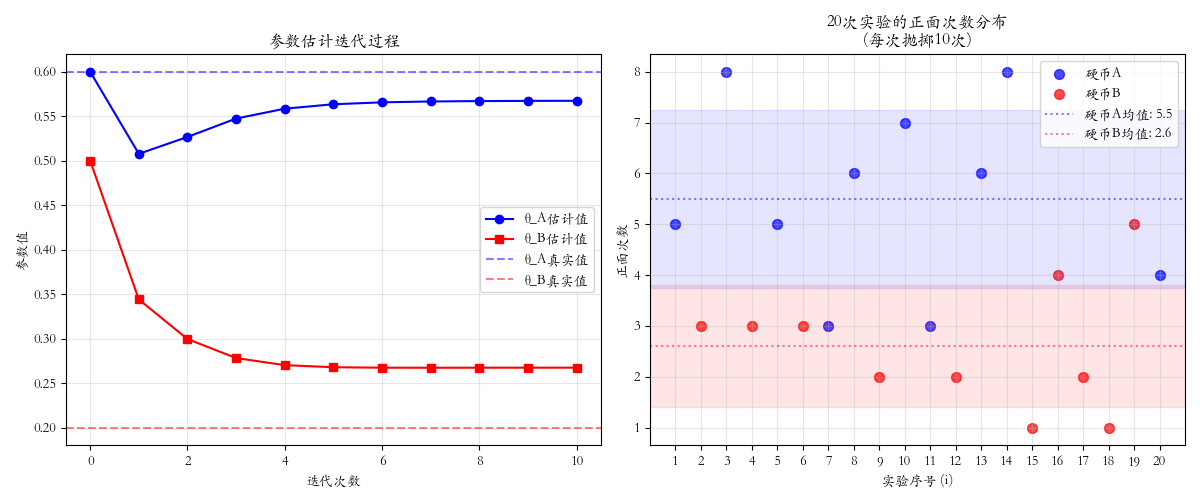
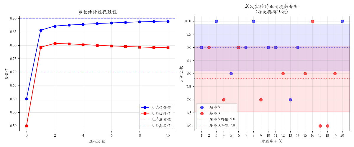
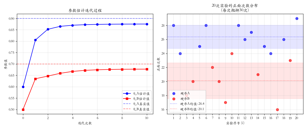
    # 4. 简单可视化
    fig, ax = plt.subplots(1, 2, figsize=(12, 5))

    # 参数迭代
    ax[0].plot(result['theta_A_history'], 'b-o', label='θ_A估计值')
    ax[0].plot(result['theta_B_history'], 'r-s', label='θ_B估计值')
    ax[0].axhline(true_theta_A, color='b', linestyle='--', alpha=0.5, label='θ_A真实值')
    ax[0].axhline(true_theta_B, color='r', linestyle='--', alpha=0.5, label='θ_B真实值')
    ax[0].set_xlabel('迭代次数')
    ax[0].set_ylabel('参数值')
    ax[0].set_title('参数估计迭代过程')
    ax[0].legend()
    ax[0].grid(True, alpha=0.3)

    # 正面次数散点图
    experiment_numbers = list(range(1, n_experiments + 1))

    # 分离硬币A和硬币B的数据
    heads_A = []
    experiments_A = []
    heads_B = []
    experiments_B = []

    for i, (h, coin) in enumerate(zip(heads_counts, true_coins)):
        if coin == 'A':
            heads_A.append(h)
            experiments_A.append(i + 1)
        else:
            heads_B.append(h)
            experiments_B.append(i + 1)

    # 绘制散点图
    ax[1].scatter(experiments_A, heads_A, color='blue', s=50, label='硬币A', alpha=0.7)
    ax[1].scatter(experiments_B, heads_B, color='red', s=50, label='硬币B', alpha=0.7)

    # 添加均值和标准差参考线
    if heads_A:
        mean_A = np.mean(heads_A)
        std_A = np.std(heads_A)
        ax[1].axhline(mean_A, color='blue', linestyle=':', alpha=0.5, label=f'硬币A均值: {mean_A:.1f}')
        ax[1].fill_between([0, n_experiments + 1],
                           [mean_A - std_A, mean_A - std_A],
                           [mean_A + std_A, mean_A + std_A],
                           color='blue', alpha=0.1)

    if heads_B:
        mean_B = np.mean(heads_B)
        std_B = np.std(heads_B)
        ax[1].axhline(mean_B, color='red', linestyle=':', alpha=0.5, label=f'硬币B均值: {mean_B:.1f}')
        ax[1].fill_between([0, n_experiments + 1],
                           [mean_B - std_B, mean_B - std_B],
                           [mean_B + std_B, mean_B + std_B],
                           color='red', alpha=0.1)

    ax[1].set_xlabel('实验序号 (i)')
    ax[1].set_ylabel('正面次数')
    ax[1].set_title(f'{n_experiments}次实验的正面次数分布\n(每次抛掷{n_tosses}次)')
    ax[1].set_xticks(range(1, n_experiments + 1))
    ax[1].legend()
    ax[1].grid(True, alpha=0.3)

    # 设置x轴范围
    ax[1].set_xlim(0, n_experiments + 1)

    plt.tight_layout()
    plt.show()


# ==================== 运行程序 ====================

if __name__ == "__main__":
    quick_demo()