机器学习与模式识别——线性回归算法

一．实验目的

• 熟悉线性回归算法的应用。
• 熟悉多项式回归算法的应用。
• 熟悉岭回归算法的应用。

二．实验内容

1.上机实验题一

房价预测问题可以看作一个线性回归问题，尝试用线性回归算法求解。利用书中图3.7线性回归的正规方程算法建立房价预测的线性模型。实现房价预测问题，实现图3.9中房价预测问题的线性回归算法。

2.上机实验题二

书本中第二章中例2.3用一个10次多项式精确地拟合了平面上的10个点，请用多项式回归算法拟合书本中例2.3的数据，实现图3.12并运行。

3.上机实验题三

书本中第二章中例2.3用一个10次多项式精确地拟合了平面上的10个点，请用岭回归算法拟合书本中例2.3的数据，实现图3.16并运行。

4.上机实验题四

糖尿病预测。

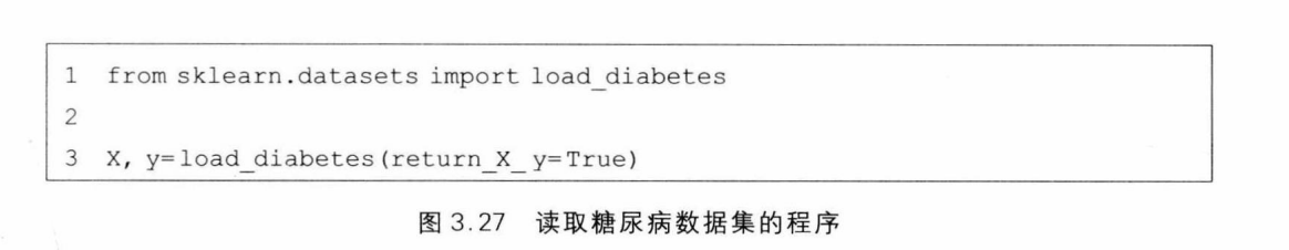
糖尿病数据集是Sklearn提供的一个标准数据集。它从442例糖尿病患者的资料中选取了10个特征----年龄、性别、体重、血压和6个血清测量值，以及这些患者在一年后疾病发展的病情量化值。糖尿病预测问题的任务是根据上述10个特征预测病情量化值。图3.27是读取糖尿病数据集的程序,其中load_diabetes函数返回特征矩阵X与标签向量y。

请用线性回归算法来完成糖尿病预测任务。

三 ． 实验 要求

1.结合上课内容，写出程序，并调试程序，要给出测试数据和实验结果。

2.整理上机步骤，总结经验和体会。

3.完成实验报告和上交源程序

四、运行代码

1.上机实验题一

首先，我们通过正规方程算法建立了一个线性模型，该模型基于房屋的特征来预测其价格。然后，我们对模型进行了训练，并在测试集上进行了预测，最后通过计算均方误差（MSE）和分数来评估模型的性能。

（1）定义线性回归类、MSE、

import numpy as np

class LinearRegression:
    def fit(self, X, y):
        self.w = np.linalg.inv(X.T.dot(X)).dot(X.T).dot(y)
        return 
    
    def predict(self, X):
        return X.dot(self.w)

def mean_squared_error(y_true, y_pred):
    return np.average((y_true - y_pred)**2, axis=0)
    
def r2_score(y_true, y_pred):
    numerator = (y_true - y_pred)**2
    denominator = (y_true - np.average(y_true, axis=0))**2
    return 1- numerator.sum(axis=0) / denominator.sum(axis=0)

（2）房价预测

import numpy as np
from sklearn.model_selection import train_test_split
from sklearn.datasets import fetch_california_housing
from sklearn.preprocessing import StandardScaler
import linear_regression.lib.linear_regression as lib

def process_features(X):
        scaler = StandardScaler()
        X = scaler.fit_transform(X)
        m, n = X.shape
        X = np.c_[np.ones((m,1)), X] 
        return X
        
housing = fetch_california_housing()
X = housing.data  
y = housing.target.reshape(-1,1)  
X_train, X_test, y_train, y_test = train_test_split(X, y, test_size=0.2, random_state=0)
X_train = process_features(X_train)
X_test = process_features(X_test)

model = lib.LinearRegression()
model.fit(X_train, y_train)  
y_pred = model.predict(X_test)
mse = lib.mean_squared_error(y_test, y_pred)
r2 = lib.r2_score(y_test, y_pred)
print("mse = {}, r2 = {}".format(mse, r2))

2.上机实验题二

首先生成了一组样本数据，并使用10次多项式来拟合这些数据。

（1）定义线性回归类、MSE、

import numpy as np

class LinearRegression:
    def fit(self, X, y):
        self.w = np.linalg.inv(X.T.dot(X)).dot(X.T).dot(y)
        return 
    
    def predict(self, X):
        return X.dot(self.w)

def mean_squared_error(y_true, y_pred):
    return np.average((y_true - y_pred)**2, axis=0)
    
def r2_score(y_true, y_pred):
    numerator = (y_true - y_pred)**2
    denominator = (y_true - np.average(y_true, axis=0))**2
    return 1- numerator.sum(axis=0) / denominator.sum(axis=0)

（2）多项式拟合平面上的10个点

import numpy as np
from sklearn.preprocessing import PolynomialFeatures
from sklearn import linear_model
import matplotlib.pyplot as plt

def generate_samples(m):
    X = 2 * (np.random.rand(m, 1) - 0.5) 
    y = X + np.random.normal(0, 0.3, (m,1))
    return X, y

np.random.seed(100)
X, y = generate_samples(10)
poly = PolynomialFeatures(degree = 10)
X_poly = poly.fit_transform(X)
model = linear_model.LinearRegression()
model.fit(X_poly, y)

plt.axis([-1, 1, -2, 2])
plt.scatter(X, y)
W = np.linspace(-1, 1, 100).reshape(100, 1)
W_poly = poly.fit_transform(W)
u = model.predict(W_poly)
plt.plot(W, u)
plt.show()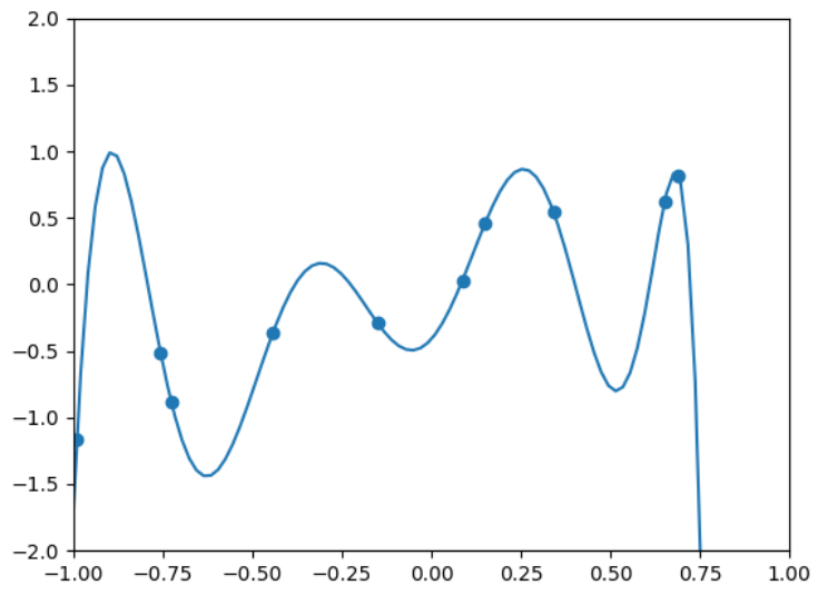

（3）多个数据点并拟合

import numpy as np
from sklearn.preprocessing import PolynomialFeatures
import matplotlib.pyplot as plt
import linear_regression.lib.linear_regression as lib

def generate_samples(m):
        X = 2 * np.random.rand(m, 1) 
        y = X**2 - 2 * X + 1 + np.random.normal(0, 0.1, (m,1))
        return X, y

np.random.seed(0)
X, y = generate_samples(100)
poly = PolynomialFeatures(degree=2)
X_poly = poly.fit_transform(X)
model = lib.LinearRegression()
model.fit(X_poly, y)

plt.figure(0)
plt.scatter(X, y)
plt.figure(1)
plt.scatter(X, y)
W = np.linspace(0, 2, 100).reshape(100, 1)
W_poly = poly.fit_transform(W)
u = model.predict(W_poly)
plt.plot(W, u)
plt.show()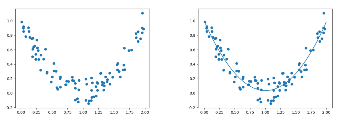

3.上机实验题三

通过添加正则化项来防止过拟合的技术。使用了一个10次多项式来拟合数据，并调整了正则化参数Lambda的值，以观察不同正则化强度下模型在训练集和测试集上的表现。

（1）定义线性回归类、MSE、

import numpy as np

class LinearRegression:
    def fit(self, X, y):
        self.w = np.linalg.inv(X.T.dot(X)).dot(X.T).dot(y)
        return 
    
    def predict(self, X):
        return X.dot(self.w)

def mean_squared_error(y_true, y_pred):
    return np.average((y_true - y_pred)**2, axis=0)
    
def r2_score(y_true, y_pred):
    numerator = (y_true - y_pred)**2
    denominator = (y_true - np.average(y_true, axis=0))**2
    return 1- numerator.sum(axis=0) / denominator.sum(axis=0)

（2）岭回归

import numpy as np

class RidgeRegression:   
    def __init__(self, Lambda):
        self.Lambda = Lambda
        
    def fit(self, X, y):
        m, n = X.shape
        r = np.diag(self.Lambda * np.ones(n))  
        self.w = np.linalg.inv(X.T.dot(X) + r).dot(X.T).dot(y)
        return 
    
    def predict(self, X):
        return X.dot(self.w)

（3）岭回归拟合

import numpy as np
from sklearn.preprocessing import PolynomialFeatures
import matplotlib.pyplot as plt
from linear_regression.lib.ridge_regression import RidgeRegression

def generate_samples(m):
    X = 2 * (np.random.rand(m, 1) - 0.5) 
    y = X + np.random.normal(0, 0.3, (m,1))
    return X, y

np.random.seed(100)
poly = PolynomialFeatures(degree = 10)

X, y = generate_samples(10)
X_poly = poly.fit_transform(X)
model = RidgeRegression(Lambda = 0.01)
model.fit(X_poly, y)

plt.scatter(X, y)
plt.axis([-1, 1, -2, 2])
W = np.linspace(-1, 1, 100).reshape(100, 1)
W_poly = poly.fit_transform(W)
u = model.predict(W_poly)
plt.plot(W, u)
plt.show()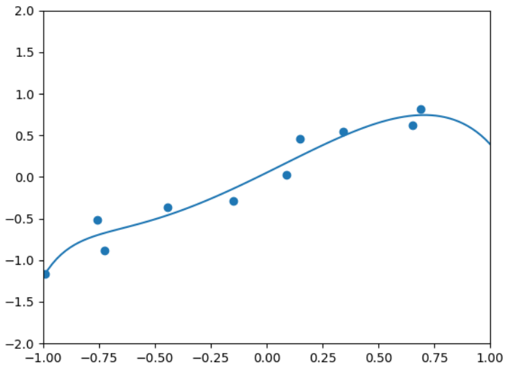

（4）岭回归在不同正则化强度下对训练集和测试集的拟合效果

import numpy as np
from sklearn.preprocessing import PolynomialFeatures
import matplotlib.pyplot as plt
import linear_regression.lib.linear_regression as lib
from linear_regression.lib.ridge_regression import RidgeRegression

def generate_samples(m):
    X = 2 * (np.random.rand(m, 1) - 0.5) 
    y = X + np.random.normal(0, 0.3, (m,1))
    return X,y

np.random.seed(100)
poly = PolynomialFeatures(degree = 10)
X_train, y_train = generate_samples(30)
X_train = poly.fit_transform(X_train)
X_test, y_test = generate_samples(100)
X_test = poly.fit_transform(X_test)

Lambdas, train_r2s, test_r2s = [], [], []
for i in range(1, 200):
    Lambda = 0.01 * i
    Lambdas.append(Lambda)
    ridge = RidgeRegression(Lambda)
    ridge.fit(X_train, y_train)
    y_train_pred = ridge.predict(X_train)
    y_test_pred = ridge.predict(X_test)
    train_r2s.append(lib.r2_score(y_train, y_train_pred))
    test_r2s.append(lib.r2_score(y_test, y_test_pred))
    
plt.figure(0)
plt.plot(Lambdas, train_r2s)
plt.figure(1)
plt.plot(Lambdas, test_r2s)
plt.show()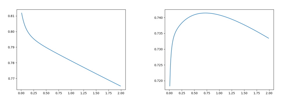

4. 上机实验题四 ------ 糖尿病预测

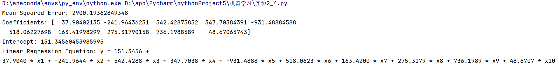
首先加载了糖尿病数据集，并将数据集分为训练集和测试集。接着，创建了一个线性回归模型并用训练集数据进行训练。训练完成后，模型对测试集进行了预测。然后，计算了预测结果的均方误差（MSE）以评估模型性能。此外，还提取了模型的系数和截距，并将它们打印出来。最后，根据这些系数和截距，构建并打印出了线性回归方程，该方程描述了各个特征与目标变量之间的关系。

# 导入所需的库
from sklearn.datasets import load_diabetes
from sklearn.model_selection import train_test_split
from sklearn.linear_model import LinearRegression
from sklearn.metrics import mean_squared_error

# 加载糖尿病数据集
X, y = load_diabetes(return_X_y=True)

# 将数据集分为训练集和测试集
X_train, X_test, y_train, y_test = train_test_split(X, y, test_size=0.2, random_state=42)

# 创建线性回归模型
model = LinearRegression()

# 训练模型
model.fit(X_train, y_train)

# 进行预测
y_pred = model.predict(X_test)

# 获取模型的系数和截距
coefficients = model.coef_
intercept = model.intercept_

# 计算预测的均方误差
mse = mean_squared_error(y_test, y_pred)
print(f'Mean Squared Error: {mse}')

# 打印模型的系数和截距
print(f'Coefficients: {model.coef_}')
print(f'Intercept: {model.intercept_}')

# 打印线性回归方程
print(f'Linear Regression Equation: y = {intercept:.4f} + ')
for i, coef in enumerate(coefficients):
    print(f'{coef:.4f} * x{i+1} + ', end='')