21_ViT凭什么挑战CNN统治地位?视觉Transformer崛起
本章目标 :打破 "CV 必须用卷积" 的思维定势。理解 Vision Transformer (ViT) 如何把图片拆成 Patch,用纯 Transformer 架构在 ImageNet 上击败 ResNet。Inductive Bias (归纳偏置) 是本章的核心关键词。
目录
- [Inductive Bias:CNN 的诅咒与祝福](#Inductive Bias:CNN 的诅咒与祝福)
- [ViT 核心操作:Patch Partition](#ViT 核心操作:Patch Partition)
- [Class Token 与位置编码](#Class Token 与位置编码)
- [CNN vs ViT:谁是未来?](#CNN vs ViT:谁是未来?)
- [实战:PyTorch 实现微型 ViT](#实战:PyTorch 实现微型 ViT)
1. Inductive Bias:CNN 的诅咒与祝福
CNN 之所以强,是因为它假设了两件事(这叫 归纳偏置 Inductive Bias):
- 局部性 (Locality):像素只和周围的像素有关(局部窗口)。
- 平移不变性 (Translation Invariance):猫在左边和右边是一样的(权重共享)。
- 祝福:这让 CNN 在小数据上也能训练得很好,收敛很快。
- 诅咒 :CNN 很难捕捉全局长距离关系。虽然堆深了能扩大感受野,但毕竟不如直接 Attention 来得直接。
ViT 的思想 :抛弃这些假设!让 Attention 自己去学像素之间的关系,哪怕相隔千里的像素也能直接交互。
代价:ViT 需要海量数据(如 JFT-300M, 3亿张图)才能"学会"这些本来由卷积提供的先验知识。
2. ViT 核心操作:Patch Partition
Transformer 的输入必须是序列 (Sequence)。怎么把一张 224 × 224 224 \times 224 224×224 的图变成序列?
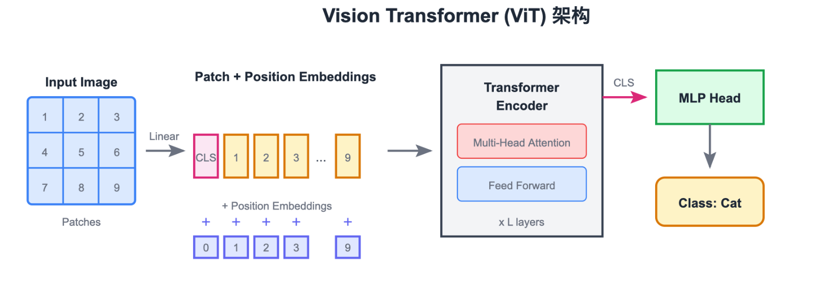
切块 (Patching) :
把图片切成 P × P P \times P P×P 的小方块(例如 16 × 16 16 \times 16 16×16)。
- 一张图变成 N = ( H / P ) × ( W / P ) N = (H/P) \times (W/P) N=(H/P)×(W/P) 个 Patch。
- 例如 224 × 224 224 \times 224 224×224,切成 196 196 196 个 16 × 16 16 \times 16 16×16 的 Patch。
- 每个 Patch 展平为一个向量(长度 16 × 16 × 3 = 768 16 \times 16 \times 3 = 768 16×16×3=768)。
- Linear Projection :通过一个线性层把这个 768 维向量映射到 D D D 维(Embedding Dimension)。
现在,图片就变成了 196 个单词。
3. Class Token 与位置编码
有了 196 个 Patch 向量后,ViT 做了两件事:
-
Class Token (CLS):
- 借用 BERT 的思想,在序列最前面加一个可学习的向量。
- 序列长度变成 196 + 1 = 197 196 + 1 = 197 196+1=197。
- Transformer 输出时,我们只取这个
[CLS]对应的输出向量去做分类。因为它通过 Attention 聚合了所有 Patch 的信息。
-
Positional Embedding:
- 因为 Transformer 没有空间概念(乱序输入结果一样),我们必须加上位置编码。
- ViT 通常使用可学习的 1D 位置编码(直接加在 Embedding 上)。
4. CNN vs ViT:谁是未来?
- 中小数据集 (ImageNet-1K, CIFAR):CNN 胜。ResNet 效率更高,更准。
- 超大数据集 (ImageNet-21K, JFT-300M):ViT 胜。ViT 的上限更高,因为它没有假设,它能学到比卷积更复杂的模式。
现在的趋势 :Hybrid(混合架构) 。
例如 Swin Transformer,引入了"局部窗口 Attention",结合了 CNN 的局部性优势和 Transformer 的全局建模能力。
5. 实战:PyTorch 实现微型 ViT
我们使用 einops 库来简化 Patch 操作(强烈推荐学习 einops)。
python
import torch
import torch.nn as nn
from einops import rearrange, repeat
from einops.layers.torch import Rearrange

# 辅助:Pre-Norm 结构的 Attention (LayerNorm 在 Attention 之前)
class PreNorm(nn.Module):
    def __init__(self, dim, fn):
        super().__init__()
        self.norm = nn.LayerNorm(dim)
        self.fn = fn
    def forward(self, x, **kwargs):
        return self.fn(self.norm(x), **kwargs)

# Feed Forward Network (GELU 激活)
class FeedForward(nn.Module):
    def __init__(self, dim, hidden_dim, dropout=0.):
        super().__init__()
        self.net = nn.Sequential(
            nn.Linear(dim, hidden_dim),
            nn.GELU(),
            nn.Dropout(dropout),
            nn.Linear(hidden_dim, dim),
            nn.Dropout(dropout)
        )
    def forward(self, x):
        return self.net(x)

# Attention (简化版)
class Attention(nn.Module):
    def __init__(self, dim, heads=8, dim_head=64, dropout=0.):
        super().__init__()
        inner_dim = dim_head * heads
        self.heads = heads
        self.scale = dim_head ** -0.5
        self.to_qkv = nn.Linear(dim, inner_dim * 3, bias = False)
        self.to_out = nn.Sequential(
            nn.Linear(inner_dim, dim),
            nn.Dropout(dropout)
        )

    def forward(self, x):
        # x: [batch, 197, dim]
        qkv = self.to_qkv(x).chunk(3, dim = -1)
        # 拆分 head
        q, k, v = map(lambda t: rearrange(t, 'b n (h d) -> b h n d', h = self.heads), qkv)

        dots = torch.matmul(q, k.transpose(-1, -2)) * self.scale
        attn = dots.softmax(dim=-1)

        out = torch.matmul(attn, v)
        out = rearrange(out, 'b h n d -> b n (h d)') # 合并 head
        return self.to_out(out)

class ViT(nn.Module):
    def __init__(self, image_size, patch_size, num_classes, dim, depth, heads, mlp_dim, channels=3):
        super().__init__()
        num_patches = (image_size // patch_size) ** 2
        patch_dim = channels * patch_size ** 2

        # 1. Patch Embedding
        self.to_patch_embedding = nn.Sequential(
            # [B, C, H, W] -> [B, N, P*P*C]
            Rearrange('b c (h p1) (w p2) -> b (h w) (p1 p2 c)', p1 = patch_size, p2 = patch_size),
            nn.Linear(patch_dim, dim),
        )

        # 2. Positional Embedding & CLS Token
        self.pos_embedding = nn.Parameter(torch.randn(1, num_patches + 1, dim))
        self.cls_token = nn.Parameter(torch.randn(1, 1, dim))

        # 3. Transformer Encoder
        self.transformer = nn.Sequential(*[
            nn.Sequential(
                PreNorm(dim, Attention(dim, heads = heads, dim_head = 64)),
                PreNorm(dim, FeedForward(dim, mlp_dim))
            ) for _ in range(depth)
        ])

        # 4. MLP Head
        self.mlp_head = nn.Sequential(
            nn.LayerNorm(dim),
            nn.Linear(dim, num_classes)
        )

    def forward(self, img):
        x = self.to_patch_embedding(img)
        b, n, _ = x.shape

        cls_tokens = repeat(self.cls_token, '() n d -> b n d', b = b)
        x = torch.cat((cls_tokens, x), dim=1) # [B, 197, Dim]
        x += self.pos_embedding[:, :(n + 1)]

        x = self.transformer(x)

        # 取 CLS token 输出
        return self.mlp_head(x[:, 0])
Part 5 (生成模型) 开启预告 :
我们已经学会了如何识别图像(判别式模型)。现在,我们要尝试扮演"造物主"的角色。
如何让神经网络画出一张世界上不存在的人脸?
自编码器 (Autoencoder) 将是我们的第一站。