基追踪法是基于冗余过完备字典下的一种信号稀疏表示方法。该方法具有可提高信号的稀疏性、实现阈值降噪和提高时频分辨率等优点。基追踪法采用表示系数的范数作为信号来度量稀疏性,通过最小化l型范数将信号稀疏表示问题定义为一类有约束的极值问题,进而转化为线性规划问题进行求解。
Speech Signal Generation and Plot
M = 100;                  % length of signal
n = 0:M-1;
s = 0.5*sin(2*pi*0.05*n); % Speech Waveform


% Plotting the speech Signal in Time Domain


figure(1)
subplot(2,1,1)
plot(n,s)
ylabel('Amplitude');
xlabel('Time');
title('Speech Waveform in Time Domain')


% Plotting the speech Signal in Frequency Domain


Y = (1/1024)*fft(s,1024);
figure(1)
subplot(2,1,2)
plot(abs(Y))
xlim([0 1024])
ylabel('Amplitude');
xlabel('Frequency');
title('Speech Waveform in Frequency Domain')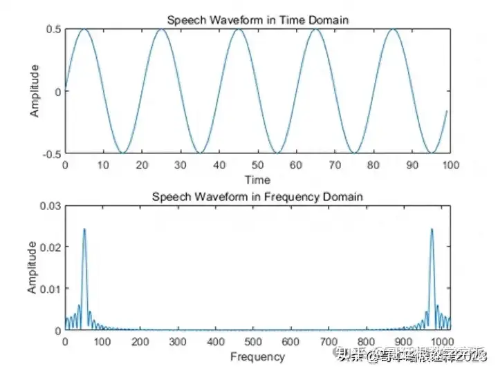
Noisy Signal Generation and Plot
w = 0.5*randn(size(s));    % w : zero-mean Gaussian noise
y = s + w;                 % y : Adding noise to speech signal


% Plotting the noisy Signal in Time Domain


figure(2)
subplot(2,1,1)
plot(y)
title('Noisy speech signal')
ylabel('Amplitude');
xlabel('Time');


% Plotting the noisy Signal in Frequency Domain


N = 2^10;                   % N : Length of Fourier coefficient vector
Y = (1/N)*fft(y,N);         % Y : Spectrum of noisy signal


figure(2)
subplot(2,1,2)
plot(abs(Y))
xlim([0 1024])
title('Fourier coefficients (FFT) of noisy signal');
xlabel('Frequency (index)')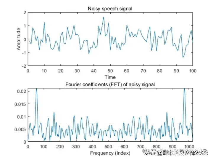
[A, AH] = MakeTransforms('DFT', 100, 2^10)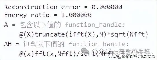
% Defining algorithm parameters


lambda = 7; % lambda : regularization parameter
Nit = 50; % Nit : number of iterations
mu = 500; % mu : ADMM parameter


% Running the  BPD algorithm


[c, cost] = BPD(y, A, AH, lambda, mu, Nit);


figure(4)
plot(cost)
title('Cost function history');
xlabel('Iteration')
it1 = 5;
del = cost(it1) - min(cost);
ylim([min(cost)-0.1*del cost(it1)])
xlim([0 Nit])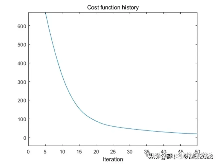
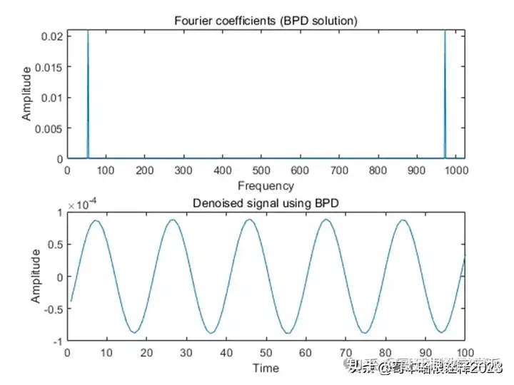
Denoising
% Plotting the denoised Signal in Frequency Domain


figure(5)
subplot(2,1,1)
plot(abs(c))
xlim([0 1024])
title('Fourier coefficients (BPD solution)');
ylabel('Amplitude')
xlabel('Frequency')


% Plotting the denoised Signal in Time Domain


figure(5)
subplot(2,1,2)
plot(ifft(c))
xlim([0 100])
title('Denoised signal using BPD');
ylabel('Amplitude')
xlabel('Time')