目录
[1. 基础图像处理工具](#1. 基础图像处理工具)
[2. 图像预处理模块](#2. 图像预处理模块)
[3. 数独轮廓检测与定位](#3. 数独轮廓检测与定位)
[4. 网格划分与单元格提取](#4. 网格划分与单元格提取)
[5. 数字特征提取](#5. 数字特征提取)
[6. 多网格处理流程](#6. 多网格处理流程)
[1. 透视变换校正算法](#1. 透视变换校正算法)
[2. 数字区域提取算法](#2. 数字区域提取算法)
[3. 多网格检测算法](#3. 多网格检测算法)
[1. 模块化设计](#1. 模块化设计)
[2. 扩展性分析](#2. 扩展性分析)
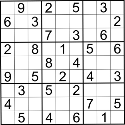
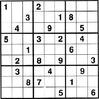
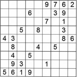
项目目的:将图片中的三个数独矩阵进行识别并一一切分出来

核心使用opencv-python进行机器视觉算法代码构建
导包
import cv2`
`import operator`
`import numpy as np`
`import os`
`from datetime import datetime`
`
工具函数构建说明
从功能模块、数据流和核心算法三个方面展开
1. 基础图像处理工具
def` `show_image(img, win='image'):`
    `"""显示图片,直到按下任意键继续"""`

`def` `show_digits(digits, color=255, withBorder=True, grid_num=1):`
    `"""将提取并处理过的81个单元格图片构成的列表显示为二维9*9大图"""`

`def` `convert_with_color(color, img):`
    `"""如果color是元组且img是灰度图,则动态地转换img为彩图"""`
`
功能:提供图像显示、多图拼接和色彩模式转换等基础工具
依赖:OpenCV的图像显示和操作函数
2. 图像预处理模块
def` `pre_process_gray(gray, skip_dilate=False):`
    `"""使用高斯模糊、自适应阈值分割和/或膨胀来暴露图像的主特征"""`
`
处理流程:高斯模糊→自适应阈值分割→形态学膨胀
关键参数:高斯核大小(9,9)、阈值方法:ADAPTIVE_THRESH_GAUSSIAN_C
3. 数独轮廓检测与定位
def` `find_corners_of_largest_polygon(bin_img):`
    `"""找出图像中面积最大轮廓的4个角点。"""`

`def` `distance_between(p1, p2):`
    `"""返回两点之间的标量距离"""`

`def` `crop_and_warp(gray, crop_rect):`
    `"""将灰度图像中由4角点围成的四边形区域裁剪出来,并将其扭曲为类似大小的正方形"""`
`
算法逻辑:
-
轮廓检测与排序(按面积降序)
-
角点定位(基于坐标和与坐标差)
-
透视变换校正
4. 网格划分与单元格提取
def` `infer_grid(square_gray):`
    `"""从正方形灰度图像推断其内部81个单元网格的位置(以等分方式)。"""`

`def` `cut_from_rect(img, rect):`
    `"""从图像中切出一个矩形ROI区域。"""`
`
划分方法:将校正后的正方形图像平均分割为9×9网格
数据结构:每个单元格由左上角和右下角坐标表示
5. 数字特征提取
def` `find_largest_feature(inp_img, scan_tl, scan_br):`
    `"""利用floodFill函数返回它所填充区域的边界框的事实,找到图像中的主特征"""`

`def` `extract_digit(bin_img, rect, size):`
    `"""从预处理后的二值方形大格子图中提取由rect指定的小单元格数字图"""`

`def` `scale_and_centre(img, size, margin=0, background=0):`
    `"""把单元格图片img经缩放且加边距,置于边长为size的新背景正方形图像中"""`
`
核心算法:
-
区域生长(floodFill)定位数字主体
-
边界框提取与裁剪
-
缩放归一化处理
6. 多网格处理流程
def` `find_sudoku_grids(image_path):`
    `"""定位图像中的所有数独图"""`

`def` `parse_multiple_grids(image_path):`
    `"""处理包含多个数独图的图像"""`

`def` `order_points(pts):`
    `"""将四个角点按左上、右上、右下、左下顺序排列"""`
`
处理流程:
-
多轮廓检测与筛选
-
角点排序与透视变换
-
网格划分与数字提取
-
结果可视化与保存
数据流分析
整个程序的数据流可以概括为:
输入:数独图像文件路径(如'sudoku2.png')
处理流程:
-
图像读取与灰度转换
-
预处理(模糊→阈值→膨胀)
-
轮廓检测与角点定位
-
透视变换校正
-
网格等分与单元格提取
-
数字区域识别与标准化
-
结果可视化与保存
输出:
校正后的数独网格图像
分割后的81个单元格图像
拼接的9×9数字大图(带网格编号)
核心算法详解
核心机器视觉方法
(一)图像预处理
高斯模糊(Gaussian Blur)原理:借助高斯核函数对图像进行卷积操作,以此降低图像噪声,平滑图像边缘。
代码体现:cv2.GaussianBlur(proc, (9, 9), 0),通过该操作减少图像中的高频噪声。
自适应阈值分割(Adaptive Thresholding)原理:依据图像局部区域的灰度值差异,动态计算阈值,从而将图像划分为前景和背景。
代码体现:
cv2.adaptiveThreshold(proc,255,cv2.ADAPTIVE_THRESH_GAUSSIAN_C, cv2.THRESH_BINARY_INV, 11, 2),
此操作能有效应对光照不均匀的情况,突出数独的边框和数字区域。
形态学操作(膨胀)原理:利用结构元素(如矩形、十字形)对图像中的前景区域进行扩张,连接邻近的区域。
代码体现:cv2.dilate(proc, kernel),这里使用特定核函数膨胀图像,用于填补数独边框的断裂处,使其轮廓更加完整。
(二)轮廓检测与几何特征分析
轮廓查找(Contour Detection)原理:通过检测图像中灰度值发生剧烈变化的像素点,形成连续的轮廓曲线,以此识别图像中的目标物体。
代码体现:cv2.findContours(processed, cv2.RETR_EXTERNAL, cv2.CHAIN_APPROX_SIMPLE),用于定位数独的外边框轮廓。
轮廓筛选与多边形逼近原理:根据轮廓的面积、顶点数量等特征筛选出符合条件的轮廓(如四边形),并使用多边形逼近轮廓的形状。
代码体现:通过面积排序和顶点数判断(len(approx) == 4)筛选数独边框,再利用cv2.approxPolyDP进行多边形逼近。
角点检测与排序原理:基于轮廓顶点的坐标和几何关系(如坐标和、坐标差),确定四边形的四个角点(左上、右上、右下、左下)。
代码体现:order_points函数通过计算坐标和与坐标差,对轮廓顶点进行排序,得到正确顺序的角点。
(三)透视变换与图像校正
透视变换(Perspective Warping)原理:根据四边形的四个角点,构建透视变换矩阵,将倾斜的数独区域校正为正矩形(正方形),消除透视畸变。
代码体现:cv2.getPerspectiveTransform(src, dst)和cv2.warpPerspective,将数独区域扭曲为规则的正方形,便于后续等分网格。
(四)区域分割与数字提取
网格划分(Grid Inference)原理:将校正后的正方形图像等分为 9×9 的网格,每个网格对应数独的一个单元格。
代码体现:infer_grid函数通过计算边长等分点,生成 81 个单元格的坐标区域。
数字区域提取(Digit Extraction)原理:运用区域生长算法(floodFill)填充数字区域,通过边界框提取数字轮廓,并进行缩放和居中处理,生成标准化的数字图像。
代码体现:find_largest_feature函数通过洪水填充找到数字的主特征区域,scale_and_centre函数将数字缩放并居中到固定尺寸(如 58×58 像素)。
1. 透视变换校正算法
def` `crop_and_warp(gray, crop_rect):`
    `# 1. 确定源点(原始四边形角点)`
`    src = np.array([top_left, top_right, bottom_right, bottom_left], dtype='float32')`

    `# 2. 计算目标正方形边长(取四边最大值)`
`    side =` `max([distance_between(p1, p2)` `for p1, p2 in pairs])`

    `# 3. 定义目标点(正方形四角)`
`    dst = np.array([[0,` `0],` `[side-1,` `0],` `[side-1, side-1],` `[0, side-1]], dtype='float32')`

    `# 4. 计算透视变换矩阵并应用`
`    m = cv2.getPerspectiveTransform(src, dst)`
`    cropped = cv2.warpPerspective(gray, m,` `(int(side),` `int(side)))`
    `return cropped`
`
数学原理:通过求解3×3透视变换矩阵,将任意四边形映射为标准矩形
关键点:角点顺序必须严格对应(左上→右上→右下→左下)
2. 数字区域提取算法
def` `extract_digit(bin_img, rect, size):`
    `# 1. 裁剪单元格区域`
`    digit = cut_from_rect(bin_img, rect)`

    `# 2. 区域生长寻找主特征`
`    flooded, bbox, seed = find_largest_feature(`
`        digit,`
        `[margin, margin],`
        `[w-margin, h-margin]`
    `)`

    `# 3. 提取边界框内的数字`
    `if valid(bbox):`
`        digit = cut_from_rect(flooded, bbox)`
        `return scale_and_centre(digit, size,` `4)`
    `else:`
        `return np.zeros((size, size), np.uint8)`
`
核心逻辑:
-
从网格中裁剪单元格
-
使用floodFill算法从中心点开始填充数字区域
-
计算填充区域的边界框
-
提取边界框内容并标准化
3. 多网格检测算法
def` `find_sudoku_grids(image_path):`
    `# 1. 图像预处理`
`    original = cv2.imread(image_path, cv2.IMREAD_GRAYSCALE)`
`    processed = pre_process_gray(original)`

    `# 2. 轮廓检测与排序`
`    contours, _ = cv2.findContours(processed, cv2.RETR_EXTERNAL, cv2.CHAIN_APPROX_SIMPLE)`
`    contours =` `sorted(contours, key=cv2.contourArea, reverse=True)`

    `# 3. 筛选四边形轮廓`
`    sudoku_grids =` `[]`
    `for contour in contours:`
`        approx = cv2.approxPolyDP(contour,` `0.02*cv2.arcLength(contour,` `True),` `True)`
        `if` `len(approx)` `==` `4:`
`            sudoku_grids.append(approx)`
    `return sudoku_grids`
`
筛选条件:
-
轮廓面积较大(排序后取前N个)
-
顶点数为4(近似四边形)
优化方向:可增加长宽比约束和角度约束提高准确性
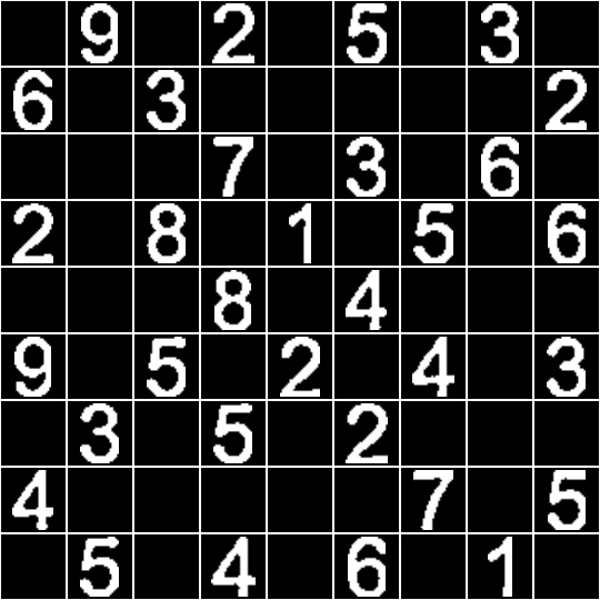
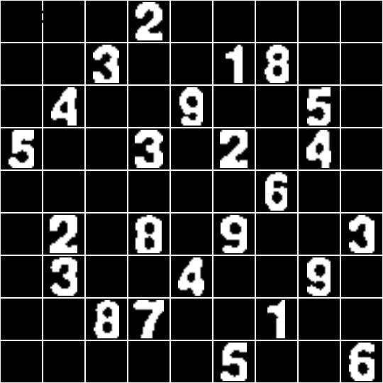
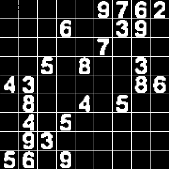
运行效果
切分结果(黑白效果图为图片增强操作):
脚本 评估
设计模式与扩展性
1. 模块化设计
各个功能模块职责单一,通过参数和返回值进行解耦
图像处理流程清晰:预处理→定位→分割→特征提取
2. 扩展性分析
优点:
可通过修改预处理参数适应不同光照条件
可替换数字提取算法(如改用深度学习模型)
多网格处理框架支持批量处理
局限性:
依赖固定网格划分(假设数独为标准9×9)
数字提取依赖简单区域生长,对复杂背景适应性差
缺乏异常处理(如未检测到数独网格的情况)
潜在优化方向
- 预处理优化:
增加直方图均衡化改善对比度
使用Canny边缘检测替代阈值分割
- 角点检测优化:
改用Harris角点检测或Shi-Tomasi算法
增加角点验证机制(如角度约束)
- 数字识别增强:
集成深度学习模型(如MNIST预训练CNN)
增加字符分类后处理(如数独规则验证)
- 性能优化:
使用Numba或Cython加速计算密集型函数
实现多线程并行处理多个数独网格
- 鲁棒性提升:
增加网格检测失败的回退策略
实现光照补偿算法适应不同环境
完整代码
import cv2`
`import operator`
`import numpy as np`
`import os`
`from datetime import datetime`

`def` `show_image(img, win='image'):`
    `"""显示图片,直到按下任意键继续"""`
`    cv2.imshow(win, img)`
`    cv2.waitKey(0)`
`    cv2.destroyAllWindows()`

`def` `show_digits(digits, color=255, withBorder=True, grid_num=1):`
    `"""将提取并处理过的81个单元格图片构成的列表显示为二维9*9大图"""`
`    rows =` `[]`
    `if withBorder:`
`        with_border =` `[cv2.copyMakeBorder(digit,` `1,` `1,` `1,` `1, cv2.BORDER_CONSTANT,` `None, color)` `for digit in digits]`
    `for i in` `range(9):`
        `if withBorder:`
`            row = np.concatenate(with_border[i *` `9:` `(i +` `1)` `*` `9], axis=1)`
        `else:`
`            row = np.concatenate(digits[i *` `9:` `(i +` `1)` `*` `9], axis=1)`
`        rows.append(row)`
`    bigImage = np.concatenate(rows, axis=0)`

    `# 在大图上添加网格编号`
    `if grid_num >` `1:`
`        font = cv2.FONT_HERSHEY_SIMPLEX`
`        cv2.putText(bigImage,` `f"Grid {grid_num}",` `(10,` `30), font,` `1,` `(0,` `0,` `255),` `2, cv2.LINE_AA)`

`    show_image(bigImage,` `f'bigImage - Grid {grid_num}')`

    `# 生成唯一文件名并保存`
`    timestamp = datetime.now().strftime("%Y%m%d_%H%M%S")`
`    filename =` `f"segmentedBigImg_grid{grid_num}_{timestamp}.jpg"`
`    cv2.imwrite(filename, bigImage)`
    `print(f"已保存数独网格 {grid_num} 到: {filename}")`

`def` `convert_with_color(color, img):`
    `"""如果color是元组且img是灰度图,则动态地转换img为彩图"""`
    `if` `len(color)` `==` `3` `and` `(img.ndim ==` `2` `or` `(img.ndim ==` `3` `and img.shape[2]` `==` `1)):`
`        img = cv2.cvtColor(img, cv2.COLOR_GRAY2BGR)`
    `return img`

`def` `pre_process_gray(gray, skip_dilate=False):`
    `"""使用高斯模糊、自适应阈值分割和/或膨胀来暴露图像的主特征"""`
`    proc = cv2.GaussianBlur(gray.copy(),` `(9,` `9),` `0)`
`    proc = cv2.adaptiveThreshold(proc,` `255, cv2.ADAPTIVE_THRESH_GAUSSIAN_C, cv2.THRESH_BINARY_INV,` `11,` `2)`
    `if` `not skip_dilate:`
`        kernel = np.array([[0.,` `1.,` `0.],` `[1.,` `1.,` `1.],` `[0.,` `1.,` `0.]], np.uint8)`
`        proc = cv2.dilate(proc, kernel)`
    `return proc`

`def` `display_points(in_img, points, radius=5, color=(0,` `0,` `255)):`
    `"""在图像上绘制彩色圆点,原图像可能是灰度图"""`
`    img = in_img.copy()`
`    img = convert_with_color(color, img)`
    `for point in points:`
`        cv2.circle(img,` `tuple(int(x)` `for x in point), radius, color,` `-1)`
    `return img`

`def` `find_corners_of_largest_polygon(bin_img):`
    `"""找出图像中面积最大轮廓的4个角点。"""`
`    contours, h = cv2.findContours(bin_img.copy(), cv2.RETR_EXTERNAL, cv2.CHAIN_APPROX_SIMPLE)`
`    contours =` `sorted(contours, key=cv2.contourArea, reverse=True)`
`    polygon = contours[0]`

`    bottom_right_idx, _ =` `max(enumerate([pt[0][0]` `+ pt[0][1]` `for pt in polygon]), key=operator.itemgetter(1))`
`    top_left_idx, _ =` `min(enumerate([pt[0][0]` `+ pt[0][1]` `for pt in polygon]), key=operator.itemgetter(1))`
`    bottom_left_idx, _ =` `min(enumerate([pt[0][0]` `- pt[0][1]` `for pt in polygon]), key=operator.itemgetter(1))`
`    top_right_idx, _ =` `max(enumerate([pt[0][0]` `- pt[0][1]` `for pt in polygon]), key=operator.itemgetter(1))`

`    points =` `[polygon[top_left_idx][0], polygon[top_right_idx][0],`
`              polygon[bottom_right_idx][0], polygon[bottom_left_idx][0]]`
`    show_image(display_points(bin_img, points),` `'4-points')`
    `return points`

`def` `distance_between(p1, p2):`
    `"""返回两点之间的标量距离"""`
`    a = p2[0]` `- p1[0]`
`    b = p2[1]` `- p1[1]`
    `return np.sqrt((a **` `2)` `+` `(b **` `2))`

`def` `crop_and_warp(gray, crop_rect):`
    `"""将灰度图像中由4角点围成的四边形区域裁剪出来,并将其扭曲为类似大小的正方形"""`
`    top_left, top_right, bottom_right, bottom_left = crop_rect[0], crop_rect[1], crop_rect[2], crop_rect[3]`
`    src = np.array([top_left, top_right, bottom_right, bottom_left], dtype='float32')`

`    side =` `max([`
`        distance_between(bottom_right, top_right),`
`        distance_between(top_left, bottom_left),`
`        distance_between(bottom_right, bottom_left),`
`        distance_between(top_left, top_right)`
    `])`

`    dst = np.array([[0,` `0],` `[side -` `1,` `0],` `[side -` `1, side -` `1],` `[0, side -` `1]], dtype='float32')`
`    m = cv2.getPerspectiveTransform(src, dst)`
`    cropped = cv2.warpPerspective(gray, m,` `(int(side),` `int(side)))`

    `# 生成唯一文件名并保存`
`    timestamp = datetime.now().strftime("%Y%m%d_%H%M%S")`
`    filename =` `f"cropped_grid_{timestamp}.png"`
`    cv2.imwrite(filename, cropped)`
    `print(f"已保存裁剪图像到: {filename}")`

`    show_image(cropped,` `'cropped')`
    `return cropped`

`def` `infer_grid(square_gray):`
    `"""从正方形灰度图像推断其内部81个单元网格的位置(以等分方式)。"""`
`    squares =` `[]`
`    side = square_gray.shape[:1][0]` `/` `9`
    `for j in` `range(9):`
        `for i in` `range(9):`
`            p1 =` `(i * side, j * side)`
`            p2 =` `((i +` `1)` `* side,` `(j +` `1)` `* side)`
`            squares.append((p1, p2))`
    `return squares`

`def` `cut_from_rect(img, rect):`
    `"""从图像中切出一个矩形ROI区域。"""`
    `return img[int(rect[0][1]):int(rect[1][1]),` `int(rect[0][0]):int(rect[1][0])]`

`def` `scale_and_centre(img, size, margin=0, background=0):`
    `"""把单元格图片img经缩放且加边距,置于边长为size的新背景正方形图像中"""`
`    h, w = img.shape[:2]`

    `def` `centre_pad(length):`
`        padAll = size - length`
        `if padAll %` `2` `==` `0:`
`            pad1 =` `int(padAll /` `2)`
`            pad2 = pad1`
        `else:`
`            pad1 =` `int(padAll /` `2)`
`            pad2 = pad1 +` `1`
        `return pad1, pad2`

    `def` `scale(r, x):`
        `return` `int(r * x)`

    `if h > w:`
`        t_pad =` `int(margin /` `2)`
`        b_pad = t_pad`
`        ratio =` `(size - margin)` `/ h`
`        w, h = scale(ratio, w), scale(ratio, h)`
`        l_pad, r_pad = centre_pad(w)`
    `else:`
`        l_pad =` `int(margin /` `2)`
`        r_pad = l_pad`
`        ratio =` `(size - margin)` `/ w`
`        w, h = scale(ratio, w), scale(ratio, h)`
`        t_pad, b_pad = centre_pad(h)`

`    img = cv2.resize(img,` `(w, h))`
`    img = cv2.copyMakeBorder(img, t_pad, b_pad, l_pad, r_pad, cv2.BORDER_CONSTANT,` `None, background)`
    `if margin %` `2` `!=` `0:`
`        img = cv2.resize(img,` `(size, size))`
    `return img`

`def` `find_largest_feature(inp_img, scan_tl, scan_br):`
    `"""利用floodFill函数返回它所填充区域的边界框的事实,找到图像中的主特征,将此结构填充为白色,其余部分降为黑色。"""`
`    img = inp_img.copy()`
`    h, w = img.shape[:2]`
`    max_area =` `0`
`    seed_point =` `(None,` `None)`

    `for x in` `range(scan_tl[0], scan_br[0]):`
        `for y in` `range(scan_tl[1], scan_br[1]):`
            `if img.item(y, x)` `==` `255` `and x < w and y < h:`
`                area = cv2.floodFill(img,` `None,` `(x, y),` `64)`
                `if area[0]` `> max_area:`
`                    max_area = area[0]`
`                    seed_point =` `(x, y)`
    `for x in` `range(w):`
        `for y in` `range(h):`
            `if img.item(y, x)` `==` `255` `and x < w and y < h:`
`                cv2.floodFill(img,` `None,` `(x, y),` `64)`

    `if` `all([p is` `not` `None` `for p in seed_point]):`
`        cv2.floodFill(img,` `None, seed_point,` `255)`
`    top, bottom, left, right = h,` `0, w,` `0`
    `for x in` `range(w):`
        `for y in` `range(h):`
            `if img.item(y, x)` `==` `64:`
`                cv2.floodFill(img,` `None,` `(x, y),` `0)`
            `if img.item(y, x)` `==` `255:`
`                top = y if y < top else top`
`                bottom = y if y > bottom else bottom`
`                left = x if x < left else left`
`                right = x if x > right else right`

`    bbox =` `[[left, top],` `[right, bottom]]`
    `return img, np.array(bbox, dtype='float32'), seed_point`

`def` `extract_digit(bin_img, rect, size):`
    `"""从预处理后的二值方形大格子图中提取由rect指定的小单元格数字图"""`
`    digit = cut_from_rect(bin_img, rect)`
`    h, w = digit.shape[:2]`
`    margin =` `int(np.mean([h, w])` `/` `2.5)`
`    flooded, bbox, seed = find_largest_feature(digit,` `[margin, margin],` `[w - margin, h - margin])`

`    w = bbox[1][0]` `- bbox[0][0]`
`    h = bbox[1][1]` `- bbox[0][1]`

    `if w >` `0` `and h >` `0` `and` `(w * h)` `>` `200:`
`        digit = cut_from_rect(flooded, bbox)`
        `return scale_and_centre(digit, size,` `4)`
    `else:`
        `return np.zeros((size, size), np.uint8)`

`def` `get_digits(square_gray, squares, size):`
    `"""提取小单元格数字,组织成数组形式"""`
`    digits =` `[]`
`    square_bin = pre_process_gray(square_gray.copy(), skip_dilate=True)`

`    color = convert_with_color((0,` `0,` `255), square_bin)`
`    h, w = color.shape[:2]`
    `for i in` `range(10):`
`        cv2.line(color,` `(0,` `int(i * h /` `9)),` `(w -` `1,` `int(i * h /` `9)),` `(0,` `0,` `255))`
`        cv2.line(color,` `(int(i * w /` `9),` `0),` `(int(i * w /` `9), h -` `1),` `(0,` `0,` `255))`
`    show_image(color,` `'drawRedLine')`

    `for square in squares:`
`        digits.append(extract_digit(square_bin, square, size))`
    `return digits`

`def` `find_sudoku_grids(image_path):`
    `"""定位图像中的所有数独图"""`
`    original = cv2.imread(image_path, cv2.IMREAD_GRAYSCALE)`
`    processed = pre_process_gray(original)`

    `# 查找轮廓`
`    contours, _ = cv2.findContours(processed, cv2.RETR_EXTERNAL, cv2.CHAIN_APPROX_SIMPLE)`
`    contours =` `sorted(contours, key=cv2.contourArea, reverse=True)`

    `# 筛选可能是数独图的轮廓(假设数独图是较大的矩形)`
`    sudoku_grids =` `[]`
    `for contour in contours:`
`        epsilon =` `0.02` `* cv2.arcLength(contour,` `True)`
`        approx = cv2.approxPolyDP(contour, epsilon,` `True)`
        `if` `len(approx)` `==` `4:`  `# 矩形`
`            sudoku_grids.append(approx)`

    `return sudoku_grids`

`def` `parse_multiple_grids(image_path):`
    `"""处理包含多个数独图的图像"""`
`    sudoku_grids = find_sudoku_grids(image_path)`
`    original = cv2.imread(image_path, cv2.IMREAD_GRAYSCALE)`

    `for i, grid in` `enumerate(sudoku_grids):`
        `print(f"Processing grid {i + 1}")`
`        corners = grid.reshape(4,` `2)`  `# 四个角点`
        `# 确保角点顺序正确(左上、右上、右下、左下)`
`        corners = order_points(corners)`
`        cropped = crop_and_warp(original, corners)`
`        squares = infer_grid(cropped)`
`        digits = get_digits(cropped, squares,` `58)`
`        show_digits(digits, withBorder=True, grid_num=i+1)`

`def` `order_points(pts):`
    `"""将四个角点按左上、右上、右下、左下顺序排列"""`
`    rect = np.zeros((4,` `2), dtype="float32")`
`    s = pts.sum(axis=1)`
`    rect[0]` `= pts[np.argmin(s)]`  `# 左上`
`    rect[2]` `= pts[np.argmax(s)]`  `# 右下`
`    diff = np.diff(pts, axis=1)`
`    rect[1]` `= pts[np.argmin(diff)]`  `# 右上`
`    rect[3]` `= pts[np.argmax(diff)]`  `# 左下`
    `return rect`

`if __name__ ==` `'__main__':`
`    image_path =` `'sudoku2.png'`
`    parse_multiple_grids(image_path)`
`
延伸用途
(一)表格识别与数据提取
应用场景:可用于答题卡识别、财务报表数字提取、手写表格内容分析等。
技术迁移:利用类似的轮廓检测和透视校正方法定位表格区域,再通过网格划分提取单元格内容,结合 OCR 技术识别文字或数字。
(二)工业检测与质量控制
应用场景:零件尺寸测量、缺陷检测(如孔洞、边缘破损)、装配完整性检查等。
技术迁移:通过轮廓分析提取零件轮廓,与标准模板对比检测缺陷;利用透视变换校正零件图像,实现高精度尺寸测量。
(三)文档图像处理
应用场景:扫描文档矫正(如弯曲页面展平)、发票 / 证件信息提取、多语言文字区域分割。
技术迁移:使用透视变换校正扫描文档的倾斜或透视畸变,结合形态学操作和轮廓检测分割文本区域,为 OCR 预处理提供高质量图像。
(四)智能安防与监控
应用场景:车牌识别(LPR)、人流量统计(通过轮廓跟踪)、异常行为检测(如遗留物品检测)。
技术迁移:通过轮廓检测定位车牌区域,结合透视变换校正车牌图像,再提取字符区域进行识别;利用轮廓跟踪算法分析监控视频中的目标运动轨迹。
(五)教育与娱乐领域
应用场景:数学作业自动批改(识别手写数字和公式)、棋盘游戏 AI(如围棋、象棋的棋盘识别)、AR/VR 互动(如手势识别中的轮廓跟踪)。
技术迁移:对数独代码中的网格分割和特征提取方法进行调整,以适应棋盘格子或手写字符的检测,结合机器学习模型实现自动评分或游戏逻辑。
(六)医学图像处理
应用场景:细胞形态分析(轮廓检测与特征提取)、显微图像分割(如组织切片中的区域划分)。
技术迁移:利用形态学操作和区域生长算法分割医学图像中的目标区域(如细胞、肿瘤),结合几何特征分析辅助疾病诊断。