- 🍨 本文为 🔗365天深度学习训练营中的学习记录博客
- 🍖 原作者: K同学啊
一、前置知识
1、VGG-16算法介绍
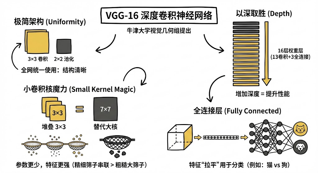
VGG-16 是由牛津大学视觉几何组(Visual Geometry Group)提出的深度卷积神经网络。它主要有以下几个核心概念:
- 极简的架构设计(Uniformity):
不同于其他网络(如 Inception)里花里胡哨的各种尺寸卷积核混用,VGG-16 全网只使用了 3 * 3 的卷积核 和 2 * 2的最大池化层。这种"强迫症"般的整齐划一,让结构非常清晰易懂。
- 以深取胜(Depth):
VGG-16 的名字来源于它有 16 层 带有权重的层(13 层卷积 + 3 层全连接)。在当时,这属于非常深的网络。它证明了**"增加网络深度"**对于提升性能至关重要。
- 小卷积核的魔力(3x3 vs 5x5/7x7):
这是 VGG 最伟大的贡献。
替代大核: 它发现,堆叠两个 3 * 3 的卷积层,其感受野(能看到的范围)等于一个 5 * 5 的卷积层;堆叠三个 3 * 3 等于一个 7 * 7。
优势: 虽然感受野一样,但堆叠小卷积核所用的参数更少 (计算量小),且因为层数多,经过了更多次非线性变换(ReLU),特征提取能力更强。
通俗说: 用几个精细的小筛子串联起来,比用一个粗糙的大筛子效果更好,还更省力。
- 全连接层(Fully Connected):
在经过多次卷积和池化将图像从"高分辨率像素"变成"低分辨率高维特征"后,最后通过 3 层全连接层将这些特征"拉平",并进行最终的分类(比如是猫还是狗)。
二、代码实现
1、设置GPU
若设备支持GPU就使用GPU,否则使用CPU
import torch
import torch.nn as nn
import matplotlib.pyplot as plt
import torchvision
import warnings
import torchvision.transforms as transforms
from torchvision import transforms, datasets
# 忽略来自 torch.cuda 的 pynvml 弃用警告
warnings.filterwarnings(
    "ignore",
    message="The pynvml package is deprecated.*",
    category=FutureWarning,
    module="torch.cuda"
)

device = torch.device("cuda" if torch.cuda.is_available() else "cpu")

device

/root/miniconda3/lib/python3.10/site-packages/torch/cuda/__init__.py:51: FutureWarning: The pynvml package is deprecated. Please install nvidia-ml-py instead. If you did not install pynvml directly, please report this to the maintainers of the package that installed pynvml for you.
  import pynvml  # type: ignore[import]

device(type='cuda')
2、数据准备
2.1、识别数据路径
import os
import pathlib

# 查看当前工作路径(确认路径是否正确)
print("当前工作路径:", os.getcwd())

# 定义数据目录(建议用绝对路径更稳妥,相对路径依赖当前工作路径)
data_dir = './data/P7周/PotatoPlants/'
data_dir = pathlib.Path(data_dir)

# 获取数据目录下的所有子路径(文件夹或文件)
data_paths = list(data_dir.glob('*'))

# 提取每个子路径的名称(即类别名,自动适配系统分隔符)
classeNames = [path.name for path in data_paths]
classeNames

当前工作路径: /root/365天训练营/Pytorch实战

['Early_blight', 'Late_blight', 'healthy']
2.2、获取数据
data_dir = './data/P7周/PotatoPlants/'

train_transforms = transforms.Compose([
    transforms.Resize([224, 224]),  # 将输入图片resize成统一尺寸
    # transforms.RandomHorizontalFlip(), # 随机水平翻转
    transforms.ToTensor(),          # 将PIL Image或numpy.ndarray转换为tensor,并归一化到[0,1]之间
    transforms.Normalize(           # 标准化处理-->转换为标准正太分布(高斯分布),使模型更容易收敛
        mean=[0.485, 0.456, 0.406],
        std=[0.229, 0.224, 0.225])  # 其中 mean=[0.485,0.456,0.406]与std=[0.229,0.224,0.225] 从数据集中随机抽样计算得到的。
])

test_transform = transforms.Compose([
    transforms.Resize([224, 224]),  # 将输入图片resize成统一尺寸
    transforms.ToTensor(),          # 将PIL Image或numpy.ndarray转换为tensor,并归一化到[0,1]之间
    transforms.Normalize(           # 标准化处理-->转换为标准正太分布(高斯分布),使模型更容易收敛
        mean=[0.485, 0.456, 0.406],
        std=[0.229, 0.224, 0.225])  # 其中 mean=[0.485,0.456,0.406]与std=[0.229,0.224,0.225] 从数据集中随机抽样计算得到的。
])

total_data = datasets.ImageFolder("./data/P7周/PotatoPlants/",transform=train_transforms)
total_data

Dataset ImageFolder
    Number of datapoints: 2152
    Root location: ./data/P7周/PotatoPlants/
    StandardTransform
Transform: Compose(
               Resize(size=[224, 224], interpolation=bilinear, max_size=None, antialias=warn)
               ToTensor()
               Normalize(mean=[0.485, 0.456, 0.406], std=[0.229, 0.224, 0.225])
           )

total_data.class_to_idx

{'Early_blight': 0, 'Late_blight': 1, 'healthy': 2}
2.3、划分数据集
train_size = int(0.8 * len(total_data))
test_size  = len(total_data) - train_size
train_dataset, test_dataset = torch.utils.data.random_split(total_data, [train_size, test_size])
train_dataset, test_dataset

batch_size = 32

train_dl = torch.utils.data.DataLoader(train_dataset,
                                           batch_size=batch_size,
                                           shuffle=True,
                                           num_workers=1)
test_dl = torch.utils.data.DataLoader(test_dataset,
                                          batch_size=batch_size,
                                          shuffle=True,
                                          num_workers=1)

for X, y in test_dl:
    print("Shape of X [N, C, H, W]: ", X.shape)
    print("Shape of y: ", y.shape, y.dtype)
    break

Shape of X [N, C, H, W]:  torch.Size([32, 3, 224, 224])
Shape of y:  torch.Size([32]) torch.int64
3、模型搭建
3.1、搭建VGG-16模型
import torch.nn.functional as F

class vgg16(nn.Module):
    def __init__(self):
        super(vgg16, self).__init__()
        # 卷积块1
        self.block1 = nn.Sequential(
            nn.Conv2d(3, 64, kernel_size=(3, 3), stride=(1, 1), padding=(1, 1)),
            nn.ReLU(),
            nn.Conv2d(64, 64, kernel_size=(3, 3), stride=(1, 1), padding=(1, 1)),
            nn.ReLU(),
            nn.MaxPool2d(kernel_size=(2, 2), stride=(2, 2))
        )
        # 卷积块2
        self.block2 = nn.Sequential(
            nn.Conv2d(64, 128, kernel_size=(3, 3), stride=(1, 1), padding=(1, 1)),
            nn.ReLU(),
            nn.Conv2d(128, 128, kernel_size=(3, 3), stride=(1, 1), padding=(1, 1)),
            nn.ReLU(),
            nn.MaxPool2d(kernel_size=(2, 2), stride=(2, 2))
        )
        # 卷积块3
        self.block3 = nn.Sequential(
            nn.Conv2d(128, 256, kernel_size=(3, 3), stride=(1, 1), padding=(1, 1)),
            nn.ReLU(),
            nn.Conv2d(256, 256, kernel_size=(3, 3), stride=(1, 1), padding=(1, 1)),
            nn.ReLU(),
            nn.Conv2d(256, 256, kernel_size=(3, 3), stride=(1, 1), padding=(1, 1)),
            nn.ReLU(),
            nn.MaxPool2d(kernel_size=(2, 2), stride=(2, 2))
        )
        # 卷积块4
        self.block4 = nn.Sequential(
            nn.Conv2d(256, 512, kernel_size=(3, 3), stride=(1, 1), padding=(1, 1)),
            nn.ReLU(),
            nn.Conv2d(512, 512, kernel_size=(3, 3), stride=(1, 1), padding=(1, 1)),
            nn.ReLU(),
            nn.Conv2d(512, 512, kernel_size=(3, 3), stride=(1, 1), padding=(1, 1)),
            nn.ReLU(),
            nn.MaxPool2d(kernel_size=(2, 2), stride=(2, 2))
        )
        # 卷积块5
        self.block5 = nn.Sequential(
            nn.Conv2d(512, 512, kernel_size=(3, 3), stride=(1, 1), padding=(1, 1)),
            nn.ReLU(),
            nn.Conv2d(512, 512, kernel_size=(3, 3), stride=(1, 1), padding=(1, 1)),
            nn.ReLU(),
            nn.Conv2d(512, 512, kernel_size=(3, 3), stride=(1, 1), padding=(1, 1)),
            nn.ReLU(),
            nn.MaxPool2d(kernel_size=(2, 2), stride=(2, 2))
        )


        # 全连接网络层,用于分类
        self.classifier = nn.Sequential(
            nn.Linear(in_features=512*7*7, out_features=4096),
            nn.ReLU(),
            nn.Linear(in_features=4096, out_features=4096),
            nn.ReLU(),
            nn.Linear(in_features=4096, out_features=3)
        )

    def forward(self, x):
        x = self.block1(x)
        x = self.block2(x)
        x = self.block3(x)
        x = self.block4(x)
        x = self.block5(x)
        x = torch.flatten(x, start_dim=1)
        x = self.classifier(x)

        return x

device = "cuda" if torch.cuda.is_available() else "cpu"
print("Using {} device".format(device))


model = vgg16().to(device)
model

Using cuda device

vgg16(
  (block1): Sequential(
    (0): Conv2d(3, 64, kernel_size=(3, 3), stride=(1, 1), padding=(1, 1))
    (1): ReLU()
    (2): Conv2d(64, 64, kernel_size=(3, 3), stride=(1, 1), padding=(1, 1))
    (3): ReLU()
    (4): MaxPool2d(kernel_size=(2, 2), stride=(2, 2), padding=0, dilation=1, ceil_mode=False)
  )
  (block2): Sequential(
    (0): Conv2d(64, 128, kernel_size=(3, 3), stride=(1, 1), padding=(1, 1))
    (1): ReLU()
    (2): Conv2d(128, 128, kernel_size=(3, 3), stride=(1, 1), padding=(1, 1))
    (3): ReLU()
    (4): MaxPool2d(kernel_size=(2, 2), stride=(2, 2), padding=0, dilation=1, ceil_mode=False)
  )
  (block3): Sequential(
    (0): Conv2d(128, 256, kernel_size=(3, 3), stride=(1, 1), padding=(1, 1))
    (1): ReLU()
    (2): Conv2d(256, 256, kernel_size=(3, 3), stride=(1, 1), padding=(1, 1))
    (3): ReLU()
    (4): Conv2d(256, 256, kernel_size=(3, 3), stride=(1, 1), padding=(1, 1))
    (5): ReLU()
    (6): MaxPool2d(kernel_size=(2, 2), stride=(2, 2), padding=0, dilation=1, ceil_mode=False)
  )
  (block4): Sequential(
    (0): Conv2d(256, 512, kernel_size=(3, 3), stride=(1, 1), padding=(1, 1))
    (1): ReLU()
    (2): Conv2d(512, 512, kernel_size=(3, 3), stride=(1, 1), padding=(1, 1))
    (3): ReLU()
    (4): Conv2d(512, 512, kernel_size=(3, 3), stride=(1, 1), padding=(1, 1))
    (5): ReLU()
    (6): MaxPool2d(kernel_size=(2, 2), stride=(2, 2), padding=0, dilation=1, ceil_mode=False)
  )
  (block5): Sequential(
    (0): Conv2d(512, 512, kernel_size=(3, 3), stride=(1, 1), padding=(1, 1))
    (1): ReLU()
    (2): Conv2d(512, 512, kernel_size=(3, 3), stride=(1, 1), padding=(1, 1))
    (3): ReLU()
    (4): Conv2d(512, 512, kernel_size=(3, 3), stride=(1, 1), padding=(1, 1))
    (5): ReLU()
    (6): MaxPool2d(kernel_size=(2, 2), stride=(2, 2), padding=0, dilation=1, ceil_mode=False)
  )
  (classifier): Sequential(
    (0): Linear(in_features=25088, out_features=4096, bias=True)
    (1): ReLU()
    (2): Linear(in_features=4096, out_features=4096, bias=True)
    (3): ReLU()
    (4): Linear(in_features=4096, out_features=3, bias=True)
  )
)
3.2、查看模型详情
# 统计模型参数量以及其他指标
import torchsummary as summary
summary.summary(model, (3, 224, 224))

----------------------------------------------------------------
        Layer (type)               Output Shape         Param #
================================================================
            Conv2d-1         [-1, 64, 224, 224]           1,792
              ReLU-2         [-1, 64, 224, 224]               0
            Conv2d-3         [-1, 64, 224, 224]          36,928
              ReLU-4         [-1, 64, 224, 224]               0
         MaxPool2d-5         [-1, 64, 112, 112]               0
            Conv2d-6        [-1, 128, 112, 112]          73,856
              ReLU-7        [-1, 128, 112, 112]               0
            Conv2d-8        [-1, 128, 112, 112]         147,584
              ReLU-9        [-1, 128, 112, 112]               0
        MaxPool2d-10          [-1, 128, 56, 56]               0
           Conv2d-11          [-1, 256, 56, 56]         295,168
             ReLU-12          [-1, 256, 56, 56]               0
           Conv2d-13          [-1, 256, 56, 56]         590,080
             ReLU-14          [-1, 256, 56, 56]               0
           Conv2d-15          [-1, 256, 56, 56]         590,080
             ReLU-16          [-1, 256, 56, 56]               0
        MaxPool2d-17          [-1, 256, 28, 28]               0
           Conv2d-18          [-1, 512, 28, 28]       1,180,160
             ReLU-19          [-1, 512, 28, 28]               0
           Conv2d-20          [-1, 512, 28, 28]       2,359,808
             ReLU-21          [-1, 512, 28, 28]               0
           Conv2d-22          [-1, 512, 28, 28]       2,359,808
             ReLU-23          [-1, 512, 28, 28]               0
        MaxPool2d-24          [-1, 512, 14, 14]               0
           Conv2d-25          [-1, 512, 14, 14]       2,359,808
             ReLU-26          [-1, 512, 14, 14]               0
           Conv2d-27          [-1, 512, 14, 14]       2,359,808
             ReLU-28          [-1, 512, 14, 14]               0
           Conv2d-29          [-1, 512, 14, 14]       2,359,808
             ReLU-30          [-1, 512, 14, 14]               0
        MaxPool2d-31            [-1, 512, 7, 7]               0
           Linear-32                 [-1, 4096]     102,764,544
             ReLU-33                 [-1, 4096]               0
           Linear-34                 [-1, 4096]      16,781,312
             ReLU-35                 [-1, 4096]               0
           Linear-36                    [-1, 3]          12,291
================================================================
Total params: 134,272,835
Trainable params: 134,272,835
Non-trainable params: 0
----------------------------------------------------------------
Input size (MB): 0.57
Forward/backward pass size (MB): 218.52
Params size (MB): 512.21
Estimated Total Size (MB): 731.30
----------------------------------------------------------------
4、训练模型
4.1、训练函数
# 训练循环
def train(dataloader, model, loss_fn, optimizer):
    size = len(dataloader.dataset)  # 训练集的大小
    num_batches = len(dataloader)   # 批次数目, (size/batch_size,向上取整)

    train_loss, train_acc = 0, 0  # 初始化训练损失和正确率


    for X, y in dataloader:  # 获取图片及其标签
        X, y = X.to(device), y.to(device)


        # 计算预测误差
        pred = model(X)          # 网络输出
        loss = loss_fn(pred, y)  # 计算网络输出和真实值之间的差距,targets为真实值,计算二者差值即为损失


        # 反向传播
        optimizer.zero_grad()  # grad属性归零
        loss.backward()        # 反向传播
        optimizer.step()       # 每一步自动更新


        # 记录acc与loss
        train_acc  += (pred.argmax(1) == y).type(torch.float).sum().item()
        train_loss += loss.item()


    train_acc  /= size
    train_loss /= num_batches

    return train_acc, train_loss
4.2、测试函数
def test (dataloader, model, loss_fn):
    size        = len(dataloader.dataset)  # 测试集的大小
    num_batches = len(dataloader)          # 批次数目, (size/batch_size,向上取整)
    test_loss, test_acc = 0, 0


    # 当不进行训练时,停止梯度更新,节省计算内存消耗
    with torch.no_grad():
        for imgs, target in dataloader:
            imgs, target = imgs.to(device), target.to(device)


            # 计算loss
            target_pred = model(imgs)
            loss        = loss_fn(target_pred, target)


            test_loss += loss.item()
            test_acc  += (target_pred.argmax(1) == target).type(torch.float).sum().item()

    test_acc  /= size
    test_loss /= num_batches

    return test_acc, test_loss
4.3、正式训练
import copy

optimizer  = torch.optim.Adam(model.parameters(), lr= 1e-4)
loss_fn    = nn.CrossEntropyLoss() # 创建损失函数

epochs     = 40

train_loss = []
train_acc  = []
test_loss  = []
test_acc   = []

best_acc = 0    # 设置一个最佳准确率,作为最佳模型的判别指标

for epoch in range(epochs):
    model.train()
    epoch_train_acc, epoch_train_loss = train(train_dl, model, loss_fn, optimizer)
    model.eval()
    epoch_test_acc, epoch_test_loss = test(test_dl, model, loss_fn)


    # 保存最佳模型到 best_model
    if epoch_test_acc > best_acc:
        best_acc   = epoch_test_acc
        best_model = copy.deepcopy(model)


    train_acc.append(epoch_train_acc)
    train_loss.append(epoch_train_loss)
    test_acc.append(epoch_test_acc)
    test_loss.append(epoch_test_loss)


    # 获取当前的学习率
    lr = optimizer.state_dict()['param_groups'][0]['lr']


    template = ('Epoch:{:2d}, Train_acc:{:.1f}%, Train_loss:{:.3f}, Test_acc:{:.1f}%, Test_loss:{:.3f}, Lr:{:.2E}')
    print(template.format(epoch+1, epoch_train_acc*100, epoch_train_loss,
                          epoch_test_acc*100, epoch_test_loss, lr))


# 保存最佳模型到文件中
PATH = './model/p7_best_model.pth'  # 保存的参数文件名
torch.save(model.state_dict(), PATH)

print('Done')

Epoch: 1, Train_acc:46.2%, Train_loss:0.941, Test_acc:47.6%, Test_loss:0.887, Lr:1.00E-04
Epoch: 2, Train_acc:46.1%, Train_loss:0.915, Test_acc:46.9%, Test_loss:0.889, Lr:1.00E-04
Epoch: 3, Train_acc:44.9%, Train_loss:0.914, Test_acc:46.9%, Test_loss:0.894, Lr:1.00E-04
Epoch: 4, Train_acc:44.9%, Train_loss:0.912, Test_acc:47.6%, Test_loss:0.871, Lr:1.00E-04
Epoch: 5, Train_acc:54.1%, Train_loss:0.847, Test_acc:68.7%, Test_loss:0.718, Lr:1.00E-04
....
Epoch:37, Train_acc:99.4%, Train_loss:0.016, Test_acc:98.1%, Test_loss:0.085, Lr:1.00E-04
Epoch:38, Train_acc:99.5%, Train_loss:0.016, Test_acc:96.5%, Test_loss:0.123, Lr:1.00E-04
Epoch:39, Train_acc:99.9%, Train_loss:0.005, Test_acc:97.4%, Test_loss:0.077, Lr:1.00E-04
Epoch:40, Train_acc:100.0%, Train_loss:0.000, Test_acc:97.9%, Test_loss:0.105, Lr:1.00E-04
Done
5、结果可视化
5.1、Loss与Accuracy图
import matplotlib.pyplot as plt
#隐藏警告
import warnings
warnings.filterwarnings("ignore")               #忽略警告信息
plt.rcParams['font.sans-serif']    = ['SimHei'] # 用来正常显示中文标签
plt.rcParams['axes.unicode_minus'] = False      # 用来正常显示负号
plt.rcParams['figure.dpi']         = 100        #分辨率

from datetime import datetime
current_time = datetime.now() # 获取当前时间

epochs_range = range(epochs)

plt.figure(figsize=(12, 3))
plt.subplot(1, 2, 1)

plt.plot(epochs_range, train_acc, label='Training Accuracy')
plt.plot(epochs_range, test_acc, label='Test Accuracy')
plt.legend(loc='lower right')
plt.title('Training and Validation Accuracy')
plt.xlabel(current_time) # 打卡请带上时间戳,否则代码截图无效

plt.subplot(1, 2, 2)
plt.plot(epochs_range, train_loss, label='Training Loss')
plt.plot(epochs_range, test_loss, label='Test Loss')
plt.legend(loc='upper right')
plt.title('Training and Validation Loss')
plt.show()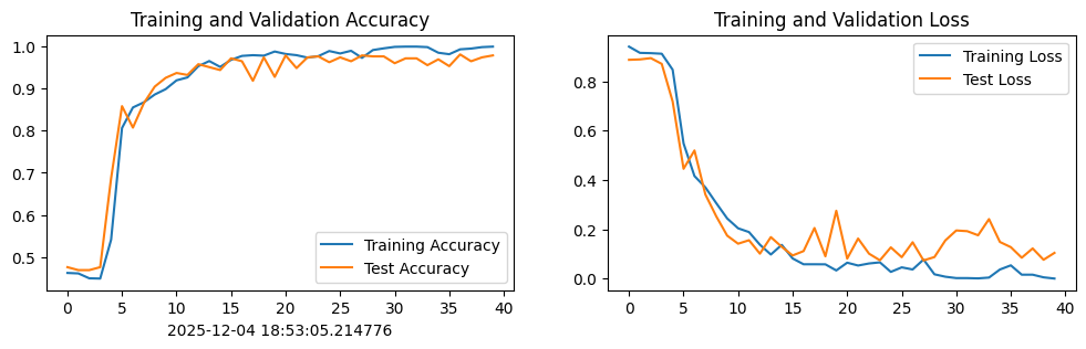
5.2、图片预测
from PIL import Image

classes = list(total_data.class_to_idx)

def predict_one_image(image_path, model, transform, classes):


    test_img = Image.open(image_path).convert('RGB')
    plt.imshow(test_img)  # 展示预测的图片

    test_img = transform(test_img)
    img = test_img.to(device).unsqueeze(0)


    model.eval()
    output = model(img)

    _,pred = torch.max(output,1)
    pred_class = classes[pred]
    print(f'预测结果是:{pred_class}')

# 预测训练集中的某张照片
predict_one_image(image_path='./data/P7周/PotatoPlants/healthy/00fc2ee5-729f-4757-8aeb-65c3355874f2___RS_HL 1864.JPG',
                  model=model,
                  transform=train_transforms,
                  classes=classes)

预测结果是:healthy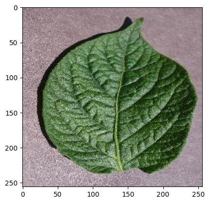
6、模型评估
best_model.eval()
epoch_test_acc, epoch_test_loss = test(test_dl, best_model, loss_fn)
epoch_test_acc, epoch_test_loss

(0.9814385150812065, 0.08554195131624251)