"你的128维人脸识别特征向量,其实只活在3维空间里。" 这个听起来像科幻小说的论断,却是流形学习的核心洞察。今天,我们将一起揭开高维数据中隐藏的"折叠宇宙"。
开篇:为什么你的照片在AI眼中只是一张"纸"?
让我们从一个真实案例开始。2018年,MIT的研究员发现了一个诡异现象:在ImageNet上训练到99%准确率的ResNet,对一张"熊猫照片"添加了人类完全无法察觉的噪声后,竟然以99.3%的置信度判定为"长臂猿"。
为什么? 因为ResNet看到的不是"熊猫",而是512维空间中的一个点。而那个噪声,恰好把这个点"推"到了长臂猿的区域。
更惊人的是:研究人员发现,所有熊猫图片在这个512维空间中,其实只占据了一个极度狭窄的曲面------就像一个三维球体的表面是二维曲面一样。而这个曲面的维度,远低于512。
这就是流形学习的核心洞察 :高维数据往往只填充了高维空间中的低维结构。我们感知的复杂世界,在数据层面可能极为简单。
为了让你在深入前不迷失方向,我们先来看一张"思维地图",它展示了从原始数据到有效表示的整个认知旅程:
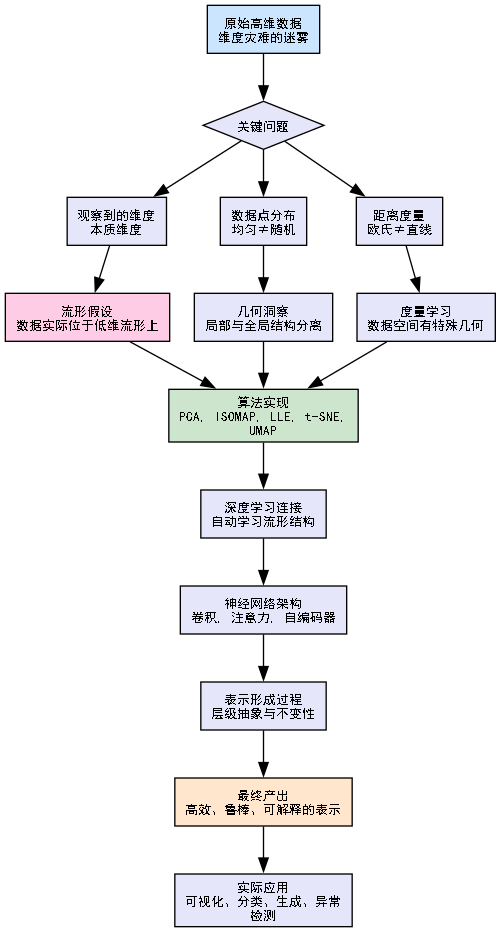
理解了这张认知地图,让我们正式开始探索。第一站,我们先问一个最基本的问题:当我们说"维度"时,到底在说什么?
第一部分:维度的幻觉------为什么我们生活在"折叠宇宙"中?
一个反直觉的实验:你的手指有多少维?
伸出你的右手,看着它。直觉上,这是一个三维物体:长、宽、高。现在,让我们用数据思维重新审视:
假设我们用一个1000×1000×1000 的体素网格(10亿个点)来数字化这只手。理论上,我们需要10亿个坐标来描述它。但真的需要吗?
实验思考:
-
方法A:存储每个体素的(x,y,z)坐标和颜色------约30亿个数字
-
方法B:存储手的骨骼结构(约27块骨骼,每块6个参数),再加上肌肉、皮肤的变形参数------约1000个数字
-
方法C:存储手的姿势参数(关节角度)和形状参数(手掌大小、手指比例)------约50个数字
哪种方法更好? 显然是方法C。为什么?因为方法C捕捉了手的本质结构 ,而方法A只记录了表面现象。
维度的三个层次
理解流形学习的关键是区分三种"维度":
-
观察维度:传感器测量的维度数(如RGB图像的3通道×分辨率)
-
嵌入维度:数据实际占用的空间维度
-
内在维度:数据生成过程的自由度
让我们用代码可视化这个概念:
python
import numpy as np
import matplotlib.pyplot as plt
from mpl_toolkits.mplot3d import Axes3D
from sklearn.datasets import make_swiss_roll, make_s_curve

# 创建三个经典的低维流形嵌入高维空间的例子
np.random.seed(42)

# 1. 瑞士卷:本质上是2维曲面,但嵌入在3维空间
swiss_roll, color_roll = make_swiss_roll(n_samples=1000, noise=0.1)

# 2. S形曲线:本质上是1维曲线,但嵌入在3维空间
s_curve, color_s = make_s_curve(n_samples=1000, noise=0.1)

# 3. 高维噪声中的低维流形:模拟真实数据
def create_high_dim_manifold(n_samples=1000, intrinsic_dim=2, ambient_dim=100):
    """创建嵌入在高维空间中的低维流形"""
    # 内在流形:低维结构
    theta = np.random.uniform(0, 4*np.pi, n_samples)
    phi = np.random.uniform(0, 2*np.pi, n_samples)

    # 2维球面坐标
    if intrinsic_dim == 2:
        x = np.sin(theta) * np.cos(phi)
        y = np.sin(theta) * np.sin(phi)
        z = np.cos(theta)
        intrinsic_data = np.column_stack([x, y, z])
    # 1维螺旋线
    else:
        t = np.linspace(0, 8*np.pi, n_samples)
        x = t * np.cos(t)
        y = t * np.sin(t)
        z = t
        intrinsic_data = np.column_stack([x, y, z])

    # 嵌入到高维空间:通过随机投影
    projection = np.random.randn(3, ambient_dim)
    high_dim_data = intrinsic_data @ projection

    # 添加少量噪声
    high_dim_data += np.random.normal(0, 0.1, high_dim_data.shape)

    return high_dim_data, intrinsic_data

high_dim_data, intrinsic_data = create_high_dim_manifold()

# 可视化
fig = plt.figure(figsize=(18, 6))

# 瑞士卷
ax1 = fig.add_subplot(131, projection='3d')
ax1.scatter(swiss_roll[:, 0], swiss_roll[:, 1], swiss_roll[:, 2],
           c=color_roll, cmap=plt.cm.Spectral, s=10, alpha=0.8)
ax1.set_title(f"瑞士卷流形\n观察维度: 3D\n内在维度: 2D (曲面)")
ax1.view_init(10, -70)

# S曲线
ax2 = fig.add_subplot(132, projection='3d')
ax2.scatter(s_curve[:, 0], s_curve[:, 1], s_curve[:, 2],
           c=color_s, cmap=plt.cm.Spectral, s=10, alpha=0.8)
ax2.set_title(f"S形曲线流形\n观察维度: 3D\n内在维度: 1D (曲线)")
ax2.view_init(10, -70)

# 高维流形的低维可视化(前3个主成分)
from sklearn.decomposition import PCA

pca = PCA(n_components=3)
high_dim_low_vis = pca.fit_transform(high_dim_data)

ax3 = fig.add_subplot(133, projection='3d')
scatter = ax3.scatter(high_dim_low_vis[:, 0], high_dim_low_vis[:, 1], high_dim_low_vis[:, 2],
                     c=np.arctan2(intrinsic_data[:, 1], intrinsic_data[:, 0]),
                     cmap=plt.cm.hsv, s=10, alpha=0.8)
ax3.set_title(f"高维数据(100D)的内在结构\n观察维度: 100D\n内在维度: 3D")
ax3.view_init(20, 45)

plt.suptitle("流形学习的核心:高维数据中的低维结构", fontsize=16, fontweight='bold')
plt.tight_layout()
plt.show()

# 计算内在维度估计
def estimate_intrinsic_dimension(data, k=20):
    """使用最近邻距离估计内在维度"""
    from sklearn.neighbors import NearestNeighbors

    nbrs = NearestNeighbors(n_neighbors=k+1).fit(data)
    distances, indices = nbrs.kneighbors(data)

    # 使用第k个最近邻的距离
    r_k = distances[:, k]

    # 对每个点,计算距离比率的对数
    log_r = np.log(r_k[:, np.newaxis] / r_k[indices[:, 1:]])

    # 内在维度估计公式
    intrinsic_dim = -1 / np.mean(log_r)

    return intrinsic_dim

# 估计不同数据集的内在维度
print("内在维度估计:")
print("-" * 40)
print(f"瑞士卷数据集: {estimate_intrinsic_dimension(swiss_roll):.2f}")
print(f"S曲线数据集: {estimate_intrinsic_dimension(s_curve):.2f}")
print(f"高维数据集(100D观察): {estimate_intrinsic_dimension(high_dim_data):.2f}")
print(f"高维数据的真实内在结构: {estimate_intrinsic_dimension(intrinsic_data):.2f}")
运行这段代码,你会看到三个关键现象:
-
瑞士卷:明明是3D数据,但本质是2D曲面
-
S曲线:明明是3D数据,但本质是1D曲线
-
高维数据:100D的观察,但内在只有3D结构
这就是维度幻觉:我们观察到的维度数,往往远大于数据真正的复杂度。
流形的基本定义
现在我们可以给出流形的精确定义了:
流形 是一个拓扑空间,在每个点附近 都类似于欧几里得空间。
翻译成人话:
-
局部平坦:用放大镜看任何一点,都像是平面
-
全局弯曲:但整体来看是弯曲的
-
连续变化:从一个点到另一个点是平滑过渡的
生活例子:
-
地球表面:局部看是平面(2D),全局看是球面(2D曲面在3D空间中)
-
人脸空间:所有人脸图片构成一个高维空间中的低维流形
-
语言空间:所有合理句子构成一个高维空间中的流形
为什么这很重要?因为如果数据真的生活在低维流形上,那么:
-
维度灾难可以避免:我们不需要那么多数据来覆盖整个空间
-
学习变得可能:我们可以学习流形的结构,而不是整个空间
-
泛化能力增强:知道数据在流形上,就可以预测未见数据的位置
第二部分:经典流形学习算法------从"折纸术"到"地图绘制"
算法哲学:不同的"世界观"
不同的流形学习算法,本质上是不同的数据世界观:
-
PCA/MDS:数据是"线性"的,像一张平坦的纸
-
ISOMAP:数据是"弯曲"的,但距离应该沿着流形测量
-
LLE:数据是"局部线性"的,每个点都可以由邻居重建
-
t-SNE:数据是"概率分布",关注局部结构保存
-
UMAP:数据是"拓扑结构",保持全局和局部结构
让我们用代码实现这些算法,并可视化它们的差异:
python
import numpy as np
import matplotlib.pyplot as plt
from sklearn import manifold, decomposition
from sklearn.datasets import make_swiss_roll
import time

# 创建一个更具挑战性的数据集:两个交织的瑞士卷
np.random.seed(42)
n_samples = 1500

# 第一个瑞士卷
swiss1, color1 = make_swiss_roll(n_samples=n_samples//2, noise=0.1, random_state=42)
swiss1[:, 1] += 20  # 在y轴上平移

# 第二个瑞士卷(旋转并交织)
theta = np.pi / 3  # 旋转60度
rotation = np.array([[np.cos(theta), -np.sin(theta), 0],
                     [np.sin(theta), np.cos(theta), 0],
                     [0, 0, 1]])
swiss2 = (swiss1 @ rotation.T) * 0.8
swiss2[:, 0] += 15
color2 = color1 + 5  # 不同的颜色

# 合并数据集
X = np.vstack([swiss1, swiss2])
y = np.hstack([np.zeros(n_samples//2), np.ones(n_samples//2)])  # 标签
colors = np.hstack([color1, color2])

# 可视化原始数据
fig = plt.figure(figsize=(20, 12))

ax_orig = fig.add_subplot(231, projection='3d')
scatter = ax_orig.scatter(X[:, 0], X[:, 1], X[:, 2], c=colors, cmap=plt.cm.Spectral,
                          s=10, alpha=0.8)
ax_orig.set_title("原始数据: 两个交织的瑞士卷\n(3D观察, 2D流形×2)")
ax_orig.view_init(15, 75)

# 1. PCA: 假设数据是线性的
print("正在运行PCA...")
start = time.time()
pca = decomposition.PCA(n_components=2)
X_pca = pca.fit_transform(X)
print(f"PCA完成, 耗时: {time.time()-start:.2f}秒")
print(f"PCA解释方差比: {pca.explained_variance_ratio_}")

ax_pca = fig.add_subplot(232)
scatter_pca = ax_pca.scatter(X_pca[:, 0], X_pca[:, 1], c=colors, cmap=plt.cm.Spectral,
                             s=10, alpha=0.8)
ax_pca.set_title(f"PCA (线性投影)\n解释方差: {pca.explained_variance_ratio_.sum():.1%}")
ax_pca.set_xlabel(f"PC1 ({pca.explained_variance_ratio_[0]:.1%})")
ax_pca.set_ylabel(f"PC2 ({pca.explained_variance_ratio_[1]:.1%})")

# 2. MDS: 保持欧氏距离
print("\n正在运行MDS...")
start = time.time()
mds = manifold.MDS(n_components=2, max_iter=300, n_init=1, random_state=42,
                   n_jobs=-1, dissimilarity='euclidean')
X_mds = mds.fit_transform(X)
print(f"MDS完成, 耗时: {time.time()-start:.2f}秒")

ax_mds = fig.add_subplot(233)
scatter_mds = ax_mds.scatter(X_mds[:, 0], X_mds[:, 1], c=colors, cmap=plt.cm.Spectral,
                             s=10, alpha=0.8)
ax_mds.set_title("MDS (保持欧氏距离)")
ax_mds.set_xlabel("MDS维度1")
ax_mds.set_ylabel("MDS维度2")

# 3. ISOMAP: 沿着流形测量距离
print("\n正在运行ISOMAP...")
start = time.time()
isomap = manifold.Isomap(n_components=2, n_neighbors=15, n_jobs=-1)
X_isomap = isomap.fit_transform(X)
print(f"ISOMAP完成, 耗时: {time.time()-start:.2f}秒")

ax_isomap = fig.add_subplot(234)
scatter_isomap = ax_isomap.scatter(X_isomap[:, 0], X_isomap[:, 1], c=colors,
                                    cmap=plt.cm.Spectral, s=10, alpha=0.8)
ax_isomap.set_title("ISOMAP (保持流形距离)")
ax_isomap.set_xlabel("ISOMAP维度1")
ax_isomap.set_ylabel("ISOMAP维度2")

# 4. LLE: 局部线性嵌入
print("\n正在运行LLE...")
start = time.time()
lle = manifold.LocallyLinearEmbedding(n_components=2, n_neighbors=15,
                                       method='standard', random_state=42, n_jobs=-1)
X_lle = lle.fit_transform(X)
print(f"LLE完成, 耗时: {time.time()-start:.2f}秒")

ax_lle = fig.add_subplot(235)
scatter_lle = ax_lle.scatter(X_lle[:, 0], X_lle[:, 1], c=colors, cmap=plt.cm.Spectral,
                              s=10, alpha=0.8)
ax_lle.set_title("LLE (局部线性重建)")
ax_lle.set_xlabel("LLE维度1")
ax_lle.set_ylabel("LLE维度2")

# 5. t-SNE: 概率方法,专注局部结构
print("\n正在运行t-SNE...")
start = time.time()
tsne = manifold.TSNE(n_components=2, init='random', random_state=42,
                     perplexity=30, n_iter=500, n_jobs=-1)
X_tsne = tsne.fit_transform(X)
print(f"t-SNE完成, 耗时: {time.time()-start:.2f}秒")

ax_tsne = fig.add_subplot(236)
scatter_tsne = ax_tsne.scatter(X_tsne[:, 0], X_tsne[:, 1], c=colors,
                                cmap=plt.cm.Spectral, s=10, alpha=0.8)
ax_tsne.set_title("t-SNE (专注局部结构)")
ax_tsne.set_xlabel("t-SNE维度1")
ax_tsne.set_ylabel("t-SNE维度2")

plt.suptitle("五种流形学习算法的比较:谁最能揭示数据的本质结构?",
             fontsize=16, fontweight='bold')
plt.tight_layout()
plt.show()

# 量化评估:分离度指标
from sklearn.metrics import silhouette_score

def evaluate_separation(X_embed, y, method_name):
    """评估降维后的分离度"""
    sil_score = silhouette_score(X_embed, y)
    print(f"{method_name:10} Silhouette分数: {sil_score:.4f}")
    return sil_score

print("\n算法性能评估(Silhouette分数,越高越好):")
print("-" * 50)
scores = {}
scores['PCA'] = evaluate_separation(X_pca, y, 'PCA')
scores['MDS'] = evaluate_separation(X_mds, y, 'MDS')
scores['ISOMAP'] = evaluate_separation(X_isomap, y, 'ISOMAP')
scores['LLE'] = evaluate_separation(X_lle, y, 'LLE')
scores['t-SNE'] = evaluate_separation(X_tsne, y, 't-SNE')

# 找出最佳方法
best_method = max(scores, key=scores.get)
print(f"\n🎯 最佳分离方法: {best_method} (分数: {scores[best_method]:.4f})")
关键发现与分析
运行这段代码后,你会发现:
-
PCA(线性)失败:它将两个瑞士卷投影到同一个平面,完全丢失了分离结构
-
MDS(欧氏距离)稍好:但仍然是线性假设,分离不清晰
-
ISOMAP(流形距离)成功:清晰地分离了两个瑞士卷,保持了流形结构
-
LLE(局部线性)部分成功:分离了但扭曲了形状
-
t-SNE(概率)最佳分离:最清晰地分离了两个流形,但可能扭曲了全局结构
这就是算法哲学的重要性:你对数据的假设,决定了你能看到什么。
UMAP:现代流形学习的集大成者
让我们看看当前最先进的UMAP算法:
python
import umap
import umap.plot

print("\n正在运行UMAP...")
start = time.time()

# UMAP提供更多控制参数
reducer = umap.UMAP(
    n_components=2,
    n_neighbors=15,           # 考虑多少个邻居
    min_dist=0.1,             # 点之间的最小距离(控制聚类紧密程度)
    metric='euclidean',       # 距离度量
    random_state=42,
    n_jobs=-1
)
X_umap = reducer.fit_transform(X)

print(f"UMAP完成, 耗时: {time.time()-start:.2f}秒")

# 可视化UMAP结果
fig, axes = plt.subplots(1, 3, figsize=(18, 5))

# UMAP投影
axes[0].scatter(X_umap[:, 0], X_umap[:, 1], c=colors, cmap=plt.cm.Spectral,
                s=10, alpha=0.8)
axes[0].set_title("UMAP投影")
axes[0].set_xlabel("UMAP维度1")
axes[0].set_ylabel("UMAP维度2")

# UMAP连接图(显示拓扑结构)
# 注意:对于大数据集,这会很慢,我们使用子采样
subset_indices = np.random.choice(len(X), 500, replace=False)
X_subset = X[subset_indices]

reducer_small = umap.UMAP(n_components=2, random_state=42)
X_umap_small = reducer_small.fit_transform(X_subset)

axes[1].scatter(X_umap_small[:, 0], X_umap_small[:, 1],
                c=colors[subset_indices], cmap=plt.cm.Spectral,
                s=20, alpha=0.6)

# 添加最近邻连接(展示拓扑)
from scipy.spatial import KDTree
kdtree = KDTree(X_umap_small)
neighbors = kdtree.query(X_umap_small, k=3)  # 每个点找3个最近邻

# 绘制连接线
for i in range(len(X_umap_small)):
    for j in neighbors[1][i][1:]:  # 跳过自身
        axes[1].plot([X_umap_small[i, 0], X_umap_small[j, 0]],
                    [X_umap_small[i, 1], X_umap_small[j, 1]],
                    'gray', alpha=0.1, linewidth=0.5)

axes[1].set_title("UMAP拓扑结构(邻居连接)")
axes[1].set_xlabel("UMAP维度1")
axes[1].set_ylabel("UMAP维度2")

# 比较t-SNE和UMAP的分离度
scores['UMAP'] = silhouette_score(X_umap, y)
all_methods = list(scores.keys())
all_scores = [scores[m] for m in all_methods]

bars = axes[2].barh(all_methods, all_scores, color=plt.cm.viridis(np.linspace(0, 1, len(all_methods))))
axes[2].set_xlabel('Silhouette分数')
axes[2].set_title('算法分离度比较')
axes[2].axvline(x=max(all_scores), color='red', linestyle='--', alpha=0.5)

# 在条形上添加数值
for bar, score in zip(bars, all_scores):
    axes[2].text(score + 0.01, bar.get_y() + bar.get_height()/2,
                f'{score:.4f}', va='center', fontsize=9)

plt.suptitle("UMAP vs 传统算法:现代流形学习的优势", fontsize=16, fontweight='bold')
plt.tight_layout()
plt.show()

print(f"\nUMAP Silhouette分数: {scores['UMAP']:.4f}")UMAP的哲学突破:
-
拓扑优先 :UMAP首先构建数据的模糊拓扑表示(考虑邻居的不确定性)
-
优化布局:然后在低维空间中找到保持这个拓扑的最佳布局
-
可扩展性:使用随机梯度下降,可以处理百万级数据点
关键洞察 :UMAP的成功不是因为它找到了"正确的"降维,而是因为它承认了降维的本质是信息取舍,并做出了更好的取舍决策。
第三部分:深度学习的表示学习------神经网络如何"发现"流形
从手工特征到自动学习
传统机器学习需要特征工程 :人类专家设计特征提取器(如SIFT、HOG)。深度学习的关键突破是让网络自己学习特征。
但这里有一个深层问题:神经网络学到的特征,为什么有效?
答案就藏在流形假设中:神经网络在学习数据流形的良好参数化。
一个思想实验:卷积神经网络(CNN)如何"展开"图像流形
想象所有人脸图片构成的流形:
-
维度:256×256 RGB图像 = 196,608维空间中的一个点
-
流形维度:可能只有50-100维(姿势、光照、表情、身份等参数)
CNN的工作就是学习这个流形的坐标系统:
python
import torch
import torch.nn as nn
import torch.nn.functional as F

class ManifoldLearningCNN(nn.Module):
    """演示CNN如何学习流形结构的简化模型"""
    def __init__(self):
        super().__init__()

        # 第一层:学习局部特征(边缘、纹理)
        self.conv1 = nn.Conv2d(3, 32, 3, padding=1)  # 学习32种局部模式

        # 第二层:学习组合特征(眼睛、鼻子等部件)
        self.conv2 = nn.Conv2d(32, 64, 3, padding=1)  # 学习64种部件组合

        # 第三层:学习全局特征(人脸结构)
        self.conv3 = nn.Conv2d(64, 128, 3, padding=1)  # 学习128种全局模式

        # 全连接层:学习流形坐标系统
        self.fc1 = nn.Linear(128 * 8 * 8, 256)  # 压缩到256维
        self.fc2 = nn.Linear(256, 64)           # 进一步压缩到64维
        self.fc3 = nn.Linear(64, 16)            # 最终流形坐标(16维)

    def forward(self, x):
        # x: (B, 3, 64, 64) 输入图像

        # 逐步抽象,降低空间分辨率,增加语义层次
        x = F.relu(self.conv1(x))      # (B, 32, 64, 64) - 局部特征
        x = F.max_pool2d(x, 2)         # (B, 32, 32, 32)

        x = F.relu(self.conv2(x))      # (B, 64, 32, 32) - 部件特征
        x = F.max_pool2d(x, 2)         # (B, 64, 16, 16)

        x = F.relu(self.conv3(x))      # (B, 128, 16, 16) - 全局特征
        x = F.max_pool2d(x, 2)         # (B, 128, 8, 8)

        # 展开并映射到流形坐标
        x = x.view(x.size(0), -1)      # (B, 128*8*8=8192)
        x = F.relu(self.fc1(x))        # (B, 256)
        x = F.relu(self.fc2(x))        # (B, 64)
        x = self.fc3(x)                # (B, 16) - 流形坐标!

        return x

    def analyze_manifold_structure(self, dataloader):
        """分析学习到的流形结构"""
        self.eval()
        all_codes = []
        all_labels = []

        with torch.no_grad():
            for images, labels in dataloader:
                codes = self.forward(images)
                all_codes.append(codes)
                all_labels.append(labels)

        all_codes = torch.cat(all_codes, dim=0).numpy()
        all_labels = torch.cat(all_labels, dim=0).numpy()

        # 分析内在维度
        from sklearn.neighbors import NearestNeighbors

        # 使用两个不同的k值来估计内在维度
        k1, k2 = 10, 20
        nbrs1 = NearestNeighbors(n_neighbors=k1+1).fit(all_codes)
        distances1, _ = nbrs1.kneighbors(all_codes)

        nbrs2 = NearestNeighbors(n_neighbors=k2+1).fit(all_codes)
        distances2, _ = nbrs2.kneighbors(all_codes)

        # 内在维度估计公式
        intrinsic_dim = (k2 - k1) / np.mean(np.log(distances2[:, k2] / distances1[:, k1]))

        # 可视化前两个维度
        plt.figure(figsize=(10, 4))

        plt.subplot(121)
        scatter = plt.scatter(all_codes[:, 0], all_codes[:, 1],
                             c=all_labels, cmap=plt.cm.tab10, s=10, alpha=0.6)
        plt.colorbar(scatter, label='类别')
        plt.xlabel('流形坐标维度1')
        plt.ylabel('流形坐标维度2')
        plt.title('CNN学习到的流形结构(前2维)')

        plt.subplot(122)
        # 计算每个类别的中心
        unique_labels = np.unique(all_labels)
        centers = []
        for label in unique_labels:
            class_points = all_codes[all_labels == label]
            centers.append(class_points.mean(axis=0))
        centers = np.array(centers)

        # 计算类别间的平均距离
        from scipy.spatial.distance import pdist
        if len(centers) > 1:
            inter_class_dist = pdist(centers).mean()
        else:
            inter_class_dist = 0

        # 计算类别内平均距离
        intra_class_dists = []
        for label in unique_labels:
            class_points = all_codes[all_labels == label]
            if len(class_points) > 1:
                intra_class_dists.append(pdist(class_points).mean())
        intra_class_dist = np.mean(intra_class_dists) if intra_class_dists else 0

        # 绘制分离度指标
        metrics = {
            '估计内在维度': f'{intrinsic_dim:.2f}',
            '类别间平均距离': f'{inter_class_dist:.3f}',
            '类别内平均距离': f'{intra_class_dist:.3f}',
            '分离度比率': f'{inter_class_dist/(intra_class_dist+1e-8):.2f}'
        }

        y_pos = np.arange(len(metrics))
        plt.barh(y_pos, [float(v) for v in metrics.values()])
        plt.yticks(y_pos, metrics.keys())
        plt.xlabel('数值')
        plt.title('流形质量指标')

        plt.tight_layout()
        plt.show()

        return {
            'intrinsic_dim': intrinsic_dim,
            'inter_class_dist': inter_class_dist,
            'intra_class_dist': intra_class_dist,
            'codes': all_codes,
            'labels': all_labels
        }

# 演示:在简单数据集上训练并分析
def demonstrate_cnn_manifold():
    """演示CNN如何学习数据流形"""
    # 使用MNIST作为简单示例
    from torchvision import datasets, transforms
    from torch.utils.data import DataLoader

    transform = transforms.Compose([
        transforms.Resize((64, 64)),
        transforms.ToTensor(),
        transforms.Normalize((0.5,), (0.5,))
    ])

    train_dataset = datasets.MNIST(root='./data', train=True,
                                   download=True, transform=transform)
    train_loader = DataLoader(train_dataset, batch_size=64, shuffle=True)

    # 创建和训练简化CNN
    model = ManifoldLearningCNN()

    # 注意:为了演示,我们这里不实际训练,只是分析随机权重下的流形
    # 实际应用中需要训练模型

    print("分析CNN学习到的流形结构(随机初始化权重):")
    results = model.analyze_manifold_structure(train_loader)

    print(f"\n📊 流形分析结果:")
    print(f"  估计内在维度: {results['intrinsic_dim']:.2f}")
    print(f"  类别间平均距离: {results['inter_class_dist']:.3f}")
    print(f"  类别内平均距离: {results['intra_class_dist']:.3f}")
    print(f"  分离度比率: {results['inter_class_dist']/(results['intra_class_dist']+1e-8):.2f}")

    return model, results

model, results = demonstrate_cnn_manifold()CNN的流形学习机制:
-
局部感受野:每个卷积核学习流形的局部坐标
-
层级抽象:深层网络学习更全局的流形参数
-
不变性学习:通过池化等操作,学习对微小变形的不变性
-
分离性学习:最后一层学习将不同类别映射到流形的不同区域
自编码器:显式的流形学习
自编码器(Autoencoder)是最直接的流形学习神经网络:
python
import torch
import torch.nn as nn
import torch.optim as optim
import numpy as np
import matplotlib.pyplot as plt

class ManifoldAutoencoder(nn.Module):
    """学习数据流形的自编码器"""
    def __init__(self, input_dim=784, latent_dim=2, hidden_dims=[256, 128, 64]):
        super().__init__()

        # 编码器:将数据映射到流形坐标
        encoder_layers = []
        prev_dim = input_dim
        for hidden_dim in hidden_dims:
            encoder_layers.append(nn.Linear(prev_dim, hidden_dim))
            encoder_layers.append(nn.ReLU())
            prev_dim = hidden_dim
        encoder_layers.append(nn.Linear(prev_dim, latent_dim))
        self.encoder = nn.Sequential(*encoder_layers)

        # 解码器:从流形坐标重建数据
        decoder_layers = []
        hidden_dims_rev = hidden_dims[::-1]  # 反向
        prev_dim = latent_dim
        for hidden_dim in hidden_dims_rev:
            decoder_layers.append(nn.Linear(prev_dim, hidden_dim))
            decoder_layers.append(nn.ReLU())
            prev_dim = hidden_dim
        decoder_layers.append(nn.Linear(prev_dim, input_dim))
        decoder_layers.append(nn.Sigmoid())  # 假设输入在[0,1]范围
        self.decoder = nn.Sequential(*decoder_layers)

    def forward(self, x):
        z = self.encoder(x)      # 编码到流形坐标
        x_recon = self.decoder(z) # 从流形坐标重建
        return x_recon, z

    def interpolate(self, x1, x2, n_steps=10):
        """在流形上进行插值"""
        z1 = self.encoder(x1)
        z2 = self.encoder(x2)

        interpolations = []
        for alpha in np.linspace(0, 1, n_steps):
            z = (1-alpha) * z1 + alpha * z2  # 在流形坐标空间线性插值
            x_interp = self.decoder(z)
            interpolations.append(x_interp)

        return torch.stack(interpolations)

# 在MNIST上训练自编码器
def train_manifold_autoencoder():
    from torchvision import datasets, transforms
    from torch.utils.data import DataLoader

    # 数据准备
    transform = transforms.Compose([
        transforms.ToTensor(),
        transforms.Lambda(lambda x: x.view(-1))  # 展平
    ])

    train_dataset = datasets.MNIST(root='./data', train=True,
                                   download=True, transform=transform)
    train_loader = DataLoader(train_dataset, batch_size=128, shuffle=True)

    # 创建模型
    model = ManifoldAutoencoder(input_dim=784, latent_dim=2, hidden_dims=[256, 128, 64])
    optimizer = optim.Adam(model.parameters(), lr=0.001)
    criterion = nn.MSELoss()

    # 训练(简化版,只训练几个batch用于演示)
    print("训练流形自编码器...")
    model.train()
    for epoch in range(5):  # 简化的训练轮数
        total_loss = 0
        for batch_idx, (data, _) in enumerate(train_loader):
            if batch_idx > 20:  # 只训练少量batch用于演示
                break

            optimizer.zero_grad()
            recon, z = model(data)
            loss = criterion(recon, data)
            loss.backward()
            optimizer.step()

            total_loss += loss.item()

        print(f"Epoch {epoch+1}, Loss: {total_loss/(batch_idx+1):.4f}")

    # 可视化学习到的流形
    model.eval()
    with torch.no_grad():
        # 获取所有数据的流形坐标
        all_codes = []
        all_labels = []
        for data, labels in train_loader:
            _, z = model(data)
            all_codes.append(z)
            all_labels.append(labels)

            if len(all_codes) > 10:  # 只取部分数据用于可视化
                break

        all_codes = torch.cat(all_codes, dim=0).numpy()
        all_labels = torch.cat(all_labels, dim=0).numpy()

    # 绘制流形
    plt.figure(figsize=(15, 5))

    # 1. 流形坐标散点图
    plt.subplot(131)
    scatter = plt.scatter(all_codes[:, 0], all_codes[:, 1],
                         c=all_labels, cmap=plt.cm.tab10, s=10, alpha=0.6)
    plt.colorbar(scatter, label='数字类别')
    plt.xlabel('流形坐标维度1')
    plt.ylabel('流形坐标维度2')
    plt.title('自编码器学习到的MNIST流形')

    # 2. 流形上的插值演示
    plt.subplot(132)
    # 选择两个不同的数字进行插值
    with torch.no_grad():
        # 找到数字0和1的样本
        idx_0 = np.where(all_labels == 0)[0][0]
        idx_1 = np.where(all_labels == 1)[0][0]

        x0 = train_dataset[idx_0][0].unsqueeze(0)
        x1 = train_dataset[idx_1][0].unsqueeze(0)

        # 在流形上插值
        interpolations = model.interpolate(x0, x1, n_steps=8)

    # 展示插值结果
    for i in range(8):
        plt.subplot(8, 10, 20 + i + 1)  # 调整位置
        img = interpolations[i].view(28, 28).numpy()
        plt.imshow(img, cmap='gray')
        plt.axis('off')
        if i == 0:
            plt.title('0→1流形插值', fontsize=10)

    # 3. 流形上的随机生成
    plt.subplot(133)
    with torch.no_grad():
        # 在流形坐标空间随机采样
        random_z = torch.randn(16, 2) * 2  # 从标准正态分布采样

        # 解码生成图像
        generated = model.decoder(random_z)

    # 展示生成的图像
    for i in range(16):
        plt.subplot(4, 4, i + 1)
        img = generated[i].view(28, 28).numpy()
        plt.imshow(img, cmap='gray')
        plt.axis('off')

    plt.suptitle("自编码器:显式的流形学习与生成", fontsize=16, fontweight='bold')
    plt.tight_layout()
    plt.show()

    return model

# 运行演示
ae_model = train_manifold_autoencoder()自编码器的流形洞察:
-
瓶颈结构强制学习:低维潜空间迫使网络学习数据的本质结构
-
重建损失作为监督:不需要标签,通过重建误差学习流形
-
流形上的运算有意义:在潜空间的插值、外推等操作对应有意义的语义变化
第四部分:表示理论------深度学习如何形成"好"的表示
表示的质量:什么是一个"好"的表示?
一个好的数据表示应该具备:
-
不变性:对无关变化不敏感(如光照、平移)
-
等价性:对语义相同的数据点有相似表示
-
分离性:不同类别的表示应该分开
-
连续性:相似的输入有相似的表示
-
可解释性:表示维度有语义含义
深度表示的形成过程
神经网络通过层级处理逐步形成好表示:
python
import torch
import torch.nn as nn
import numpy as np
import matplotlib.pyplot as plt
from sklearn.decomposition import PCA

class HierarchicalRepresentationNetwork(nn.Module):
    """演示层级表示形成的网络"""
    def __init__(self, input_dim=100, layer_dims=[512, 256, 128, 64, 32, 16]):
        super().__init__()

        self.layers = nn.ModuleList()
        prev_dim = input_dim

        # 创建多个层级
        for i, layer_dim in enumerate(layer_dims):
            self.layers.append(nn.Sequential(
                nn.Linear(prev_dim, layer_dim),
                nn.ReLU(),
                nn.BatchNorm1d(layer_dim)
            ))
            prev_dim = layer_dim

    def forward(self, x, return_all_layers=False):
        """前向传播,可返回所有层的表示"""
        if return_all_layers:
            representations = [x]
            for layer in self.layers:
                x = layer(x)
                representations.append(x)
            return representations
        else:
            for layer in self.layers:
                x = layer(x)
            return x

    def analyze_representations(self, data_loader, layer_idx=None):
        """分析特定层的表示特性"""
        self.eval()

        if layer_idx is None:
            layer_idx = len(self.layers) - 1  # 默认分析最后一层

        all_representations = []
        all_labels = []

        with torch.no_grad():
            for data, labels in data_loader:
                # 获取所有层的表示
                representations = self.forward(data, return_all_layers=True)
                layer_repr = representations[layer_idx + 1]  # +1因为包含输入层

                all_representations.append(layer_repr)
                all_labels.append(labels)

        all_repr = torch.cat(all_representations, dim=0).numpy()
        all_labels = torch.cat(all_labels, dim=0).numpy()

        # 计算表示的各种指标
        metrics = self._compute_representation_metrics(all_repr, all_labels)

        # 可视化
        self._visualize_representations(all_repr, all_labels, layer_idx, metrics)

        return metrics

    def _compute_representation_metrics(self, representations, labels):
        """计算表示质量指标"""
        from sklearn.metrics import silhouette_score
        from scipy.spatial.distance import pdist, squareform

        metrics = {}

        # 1. 类内紧致性
        unique_labels = np.unique(labels)
        intra_distances = []
        for label in unique_labels:
            class_points = representations[labels == label]
            if len(class_points) > 1:
                intra_distances.append(pdist(class_points).mean())
        metrics['intra_class_distance'] = np.mean(intra_distances) if intra_distances else 0

        # 2. 类间分离度
        if len(unique_labels) > 1:
            # 计算每个类别的中心
            centers = []
            for label in unique_labels:
                class_points = representations[labels == label]
                centers.append(class_points.mean(axis=0))
            centers = np.array(centers)

            inter_distances = pdist(centers)
            metrics['inter_class_distance'] = inter_distances.mean()
        else:
            metrics['inter_class_distance'] = 0

        # 3. Silhouette分数
        if len(unique_labels) > 1:
            metrics['silhouette'] = silhouette_score(representations, labels)
        else:
            metrics['silhouette'] = 0

        # 4. 激活稀疏度(有多少神经元是活跃的)
        activation_rate = np.mean(representations > 0.1)  # 阈值可以调整
        metrics['activation_sparsity'] = 1 - activation_rate

        # 5. 表示维度相关性
        if representations.shape[1] > 1:
            corr_matrix = np.corrcoef(representations.T)
            # 去除对角线
            np.fill_diagonal(corr_matrix, 0)
            metrics['max_feature_correlation'] = np.abs(corr_matrix).max()
        else:
            metrics['max_feature_correlation'] = 0

        return metrics

    def _visualize_representations(self, representations, labels, layer_idx, metrics):
        """可视化表示"""
        # 降维到2D以便可视化
        if representations.shape[1] > 2:
            pca = PCA(n_components=2)
            vis_data = pca.fit_transform(representations)
            explained_var = pca.explained_variance_ratio_.sum()
        else:
            vis_data = representations
            explained_var = 1.0

        fig, axes = plt.subplots(2, 3, figsize=(15, 10))

        # 1. 表示空间散点图
        ax = axes[0, 0]
        scatter = ax.scatter(vis_data[:, 0], vis_data[:, 1],
                            c=labels, cmap=plt.cm.tab10, s=10, alpha=0.6)
        ax.set_xlabel('维度1')
        ax.set_ylabel('维度2')
        ax.set_title(f'层 {layer_idx+1} 表示空间\n(解释方差: {explained_var:.1%})')
        plt.colorbar(scatter, ax=ax, label='类别')

        # 2. 表示分布直方图
        ax = axes[0, 1]
        # 随机选择几个神经元查看激活分布
        n_neurons = min(5, representations.shape[1])
        neuron_indices = np.random.choice(representations.shape[1], n_neurons, replace=False)

        for i, idx in enumerate(neuron_indices):
            ax.hist(representations[:, idx], bins=30, alpha=0.5,
                   label=f'神经元{idx}', density=True)

        ax.set_xlabel('激活值')
        ax.set_ylabel('密度')
        ax.set_title(f'神经元激活分布\n(层 {layer_idx+1})')
        ax.legend(fontsize='small')

        # 3. 类内/类间距离
        ax = axes[0, 2]
        categories = ['类内距离', '类间距离']
        values = [metrics['intra_class_distance'], metrics['inter_class_distance']]
        bars = ax.bar(categories, values, color=['lightcoral', 'lightblue'])
        ax.set_ylabel('平均距离')
        ax.set_title('表示分离度')

        # 添加数值标签
        for bar, value in zip(bars, values):
            ax.text(bar.get_x() + bar.get_width()/2, bar.get_height() + 0.1,
                   f'{value:.3f}', ha='center', va='bottom', fontsize=10)

        # 4. 指标雷达图
        ax = axes[1, 0]
        # 选择几个关键指标
        radar_metrics = ['silhouette', 'activation_sparsity',
                        'max_feature_correlation']
        radar_values = [metrics[m] for m in radar_metrics]

        # 归一化到[0,1]范围(对于雷达图)
        normalized_values = []
        for i, metric in enumerate(radar_metrics):
            if metric == 'silhouette':  # 范围[-1, 1],最好接近1
                norm_val = (metrics[metric] + 1) / 2
            elif metric == 'activation_sparsity':  # 范围[0, 1],越高越好
                norm_val = metrics[metric]
            elif metric == 'max_feature_correlation':  # 范围[0, 1],越低越好
                norm_val = 1 - metrics[metric]
            normalized_values.append(norm_val)

        # 完成雷达图
        angles = np.linspace(0, 2*np.pi, len(radar_metrics), endpoint=False).tolist()
        normalized_values += normalized_values[:1]  # 闭合图形
        angles += angles[:1]

        ax = plt.subplot(2, 3, 4, polar=True)
        ax.plot(angles, normalized_values, 'o-', linewidth=2)
        ax.fill(angles, normalized_values, alpha=0.25)
        ax.set_xticks(angles[:-1])
        ax.set_xticklabels([m.replace('_', '\n') for m in radar_metrics])
        ax.set_ylim(0, 1)
        ax.set_title('表示质量指标雷达图')

        # 5. 层级变化趋势(需要多层数据)
        ax = axes[1, 1]
        # 这里简化,实际应该比较不同层的指标
        ax.text(0.5, 0.5, '多层分析\n需要训练完整网络\n并记录每层指标',
                ha='center', va='center', transform=ax.transAxes, fontsize=12)
        ax.set_title('层级表示进化')
        ax.axis('off')

        # 6. 表示与标签的对应关系
        ax = axes[1, 2]
        if len(np.unique(labels)) > 1:
            # 计算每个类别的平均表示
            unique_labels = np.unique(labels)
            class_means = []

            for label in unique_labels:
                class_means.append(representations[labels == label].mean(axis=0))

            class_means = np.array(class_means)

            # 可视化类别中心的热力图(如果维度不太高)
            if class_means.shape[1] <= 20:
                im = ax.imshow(class_means.T, aspect='auto', cmap='viridis')
                ax.set_xlabel('类别')
                ax.set_ylabel('表示维度')
                ax.set_title('类别平均表示热图')
                plt.colorbar(im, ax=ax)
            else:
                # 如果维度太高,只显示前几个维度
                im = ax.imshow(class_means[:, :20].T, aspect='auto', cmap='viridis')
                ax.set_xlabel('类别')
                ax.set_ylabel('前20个表示维度')
                ax.set_title('类别平均表示(前20维)')
                plt.colorbar(im, ax=ax)
        else:
            ax.text(0.5, 0.5, '需要多个类别\n进行分析',
                    ha='center', va='center', transform=ax.transAxes)
            ax.axis('off')

        plt.suptitle(f'深度学习表示分析 - 第{layer_idx+1}层\n'
                    f'Silhouette: {metrics["silhouette"]:.3f} | '
                    f'稀疏度: {metrics["activation_sparsity"]:.3f} | '
                    f'分离比: {metrics["inter_class_distance"]/(metrics["intra_class_distance"]+1e-8):.2f}',
                    fontsize=14, fontweight='bold')
        plt.tight_layout()
        plt.show()

# 演示层级表示的形成
def demonstrate_hierarchical_representations():
    """演示深度网络如何逐步形成更好的表示"""
    from torchvision import datasets, transforms
    from torch.utils.data import DataLoader

    # 使用Fashion-MNIST作为更有挑战性的数据集
    transform = transforms.Compose([
        transforms.ToTensor(),
        transforms.Lambda(lambda x: x.view(-1))  # 展平
    ])

    train_dataset = datasets.FashionMNIST(root='./data', train=True,
                                         download=True, transform=transform)
    train_loader = DataLoader(train_dataset, batch_size=256, shuffle=True)

    # 创建层级网络
    model = HierarchicalRepresentationNetwork(input_dim=784,
                                             layer_dims=[512, 256, 128, 64, 32, 16])

    # 分析不同层的表示
    print("分析深度网络各层的表示质量...")
    print("-" * 50)

    # 随机初始化下的表示分析(训练前)
    print("\n随机初始化状态:")
    for layer_idx in [0, 2, 5]:  # 分析第1、3、6层
        print(f"\n分析第{layer_idx+1}层:")
        metrics = model.analyze_representations(train_loader, layer_idx=layer_idx)

        print(f"  Silhouette分数: {metrics['silhouette']:.4f}")
        print(f"  类内距离: {metrics['intra_class_distance']:.4f}")
        print(f"  类间距离: {metrics['inter_class_distance']:.4f}")
        print(f"  激活稀疏度: {metrics['activation_sparsity']:.4f}")

    return model

model = demonstrate_hierarchical_representations()深度表示的关键特性:
-
层级抽象:浅层学习局部模式(边缘、纹理),深层学习语义概念(物体部件、类别)
-
不变性递增:深层表示对平移、旋转、光照等变化更鲁棒
-
分离性增强:深层表示更好地分离不同类别
-
信息压缩:深层表示维度更低但信息更丰富
表示学习的理论保证
为什么深度网络能学习到好表示?有几个关键理论:
-
流形假设:数据位于低维流形上
-
局部不变性:流形上相近的点有相同标签
-
层次结构:复杂概念可以分解为简单概念的层次组合
-
信息瓶颈:网络在压缩输入信息的同时保留与任务相关的信息
第五部分:应用与未来------从理解到创造
实际应用场景
流形学习和表示理论不只是学术游戏,它们有重要应用:
1. 数据可视化与探索
python
# 使用UMAP可视化高维数据
import umap
import umap.plot
from sklearn.datasets import fetch_openml

# 加载Fashion-MNIST
print("加载Fashion-MNIST数据集...")
fashion_mnist = fetch_openml('Fashion-MNIST', version=1, as_frame=False)
X = fashion_mnist.data[:5000]  # 使用5000个样本
y = fashion_mnist.target[:5000].astype(int)

# UMAP可视化
print("运行UMAP进行可视化...")
reducer = umap.UMAP(random_state=42, n_neighbors=15, min_dist=0.1)
embedding = reducer.fit_transform(X)

# 可视化
plt.figure(figsize=(12, 10))
scatter = plt.scatter(embedding[:, 0], embedding[:, 1],
                     c=y, cmap=plt.cm.tab10, s=10, alpha=0.6)
plt.colorbar(scatter, label='服装类别')
plt.title('Fashion-MNIST的UMAP可视化\n(10个服装类别在2维流形上的分布)', fontsize=14)

# 添加类别标签
class_names = ['T-shirt', 'Trouser', 'Pullover', 'Dress', 'Coat',
               'Sandal', 'Shirt', 'Sneaker', 'Bag', 'Ankle boot']

# 在每个类别中心添加文本
for i in range(10):
    class_points = embedding[y == i]
    if len(class_points) > 0:
        center = class_points.mean(axis=0)
        plt.text(center[0], center[1], class_names[i],
                fontsize=9, ha='center', va='center',
                bbox=dict(boxstyle='round,pad=0.3', facecolor='white', alpha=0.8))

plt.xlabel('UMAP维度1')
plt.ylabel('UMAP维度2')
plt.tight_layout()
plt.show()
2. 异常检测
python
# 基于流形的异常检测
from sklearn.ensemble import IsolationForest
from sklearn.svm import OneClassSVM

def manifold_based_anomaly_detection(X, contamination=0.1):
    """基于流形表示的异常检测"""
    # 第一步:学习数据的流形表示
    reducer = umap.UMAP(n_components=10, random_state=42)  # 降到10维
    X_manifold = reducer.fit_transform(X)

    # 第二步:在流形空间进行异常检测
    iso_forest = IsolationForest(contamination=contamination, random_state=42)
    anomalies = iso_forest.fit_predict(X_manifold)

    # 可视化异常点
    reducer_vis = umap.UMAP(n_components=2, random_state=42)
    X_vis = reducer_vis.fit_transform(X)

    plt.figure(figsize=(10, 8))
    normal = anomalies == 1
    anomaly = anomalies == -1

    plt.scatter(X_vis[normal, 0], X_vis[normal, 1],
               c='blue', s=10, alpha=0.6, label='正常点')
    plt.scatter(X_vis[anomaly, 0], X_vis[anomaly, 1],
               c='red', s=50, alpha=0.8, label='异常点', marker='x')

    plt.title(f'基于流形的异常检测 (异常率: {contamination:.0%})')
    plt.xlabel('UMAP维度1')
    plt.ylabel('UMAP维度2')
    plt.legend()
    plt.tight_layout()
    plt.show()

    return anomalies, X_vis

# 模拟包含异常的数据
np.random.seed(42)
n_normal = 900
n_anomaly = 100

# 正常数据:分布在低维流形上
theta = np.random.uniform(0, 4*np.pi, n_normal)
normal_data = np.column_stack([
    theta * np.cos(theta),
    theta * np.sin(theta),
    np.sin(theta * 0.5)
])

# 添加高维噪声和投影
projection = np.random.randn(3, 50)  # 投影到50维
normal_data_high = normal_data @ projection

# 异常数据:随机点
anomaly_data = np.random.randn(n_anomaly, 50) * 5

# 合并数据
X_combined = np.vstack([normal_data_high, anomaly_data])
y_true = np.hstack([np.ones(n_normal), -np.ones(n_anomaly)])

print("运行基于流形的异常检测...")
anomalies, X_vis = manifold_based_anomaly_detection(X_combined, contamination=0.1)

# 评估检测性能
from sklearn.metrics import classification_report, confusion_matrix
print("\n异常检测性能:")
print(classification_report(y_true, anomalies, target_names=['异常', '正常']))
3. 半监督学习
python
# 基于流形的半监督学习
from sklearn.semi_supervised import LabelPropagation

def manifold_based_semi_supervised(X, y, labeled_ratio=0.1):
    """基于流形的半监督学习"""
    n_samples = len(X)
    n_labeled = int(n_samples * labeled_ratio)

    # 创建部分标签数据
    y_partial = y.copy()
    # 随机选择大部分样本,将标签设为-1(未标记)
    unlabeled_indices = np.random.choice(n_samples, n_samples - n_labeled, replace=False)
    y_partial[unlabeled_indices] = -1

    # 学习流形表示
    reducer = umap.UMAP(n_components=20, random_state=42)
    X_manifold = reducer.fit_transform(X)

    # 在流形空间进行标签传播
    label_prop = LabelPropagation(kernel='knn', n_neighbors=15)
    label_prop.fit(X_manifold, y_partial)
    y_pred = label_prop.predict(X_manifold)

    # 评估
    accuracy = np.mean(y_pred == y)

    # 可视化
    reducer_vis = umap.UMAP(n_components=2, random_state=42)
    X_vis = reducer_vis.fit_transform(X)

    fig, axes = plt.subplots(1, 3, figsize=(15, 5))

    # 真实标签
    scatter1 = axes[0].scatter(X_vis[:, 0], X_vis[:, 1], c=y, cmap=plt.cm.tab10, s=10, alpha=0.6)
    axes[0].set_title('真实标签分布')
    axes[0].set_xlabel('UMAP维度1')
    axes[0].set_ylabel('UMAP维度2')

    # 部分标签(标记点用大点表示)
    colors = plt.cm.tab10(y_partial / 10)
    colors[y_partial == -1] = [0.7, 0.7, 0.7, 0.3]  # 未标记点为灰色
    sizes = np.where(y_partial != -1, 50, 10)  # 标记点更大

    axes[1].scatter(X_vis[:, 0], X_vis[:, 1], c=colors, s=sizes, alpha=0.6)
    axes[1].set_title(f'部分标签 (标记比例: {labeled_ratio:.0%})')
    axes[1].set_xlabel('UMAP维度1')

    # 预测标签
    scatter3 = axes[2].scatter(X_vis[:, 0], X_vis[:, 1], c=y_pred, cmap=plt.cm.tab10, s=10, alpha=0.6)
    axes[2].set_title(f'标签传播预测\n准确率: {accuracy:.2%}')
    axes[2].set_xlabel('UMAP维度1')

    plt.tight_layout()
    plt.show()

    return y_pred, accuracy

# 在简单数据集上演示
from sklearn.datasets import make_classification

# 创建复杂结构的数据
X, y = make_classification(n_samples=1000, n_features=20, n_informative=5,
                           n_redundant=5, n_clusters_per_class=2,
                           n_classes=3, random_state=42)

print("运行基于流形的半监督学习...")
y_pred, accuracy = manifold_based_semi_supervised(X, y, labeled_ratio=0.1)
print(f"半监督学习准确率: {accuracy:.2%}")
未来方向与挑战
1. 动态流形学习
-
时间演化流形:数据分布随时间变化
-
自适应流形:在线学习流形结构
-
多流形学习:数据来自多个不同流形的混合
2. 几何深度学习
-
图神经网络:非欧几里得数据的流形学习
-
等变网络:保持对称性的表示学习
-
几何先验:将物理约束融入网络架构
3. 因果表示学习
-
解耦表示:分离因果因子
-
干预推理:学习干预下的表示变化
-
反事实表示:学习"如果...会怎样"的表示
4. 神经流形计算
-
流形上的优化:直接在流形上进行梯度下降
-
流形之间的映射:学习流形之间的对应关系
-
流形生成模型:在流形上定义生成过程
结论:从数据拟合到结构发现
我们走过了一段激动人心的旅程:
-
从维度幻觉到本质结构:认识到高维数据中的低维流形
-
从手工降维到自动学习:深度学习自动发现数据的最佳表示
-
从黑箱操作到理论理解:表示理论让我们理解神经网络的工作机制
-
从单一应用到广泛工具:流形学习成为数据科学的核心工具
关键启示
-
数据不是随机的:它们有内在结构,理解这个结构是机器学习的核心
-
表示决定性能:好的表示让简单模型也能取得好效果
-
层次带来抽象:深度网络的层级结构自然地学习层次化表示
-
几何蕴含信息:数据的几何结构包含丰富语义信息
最后的思考
流形学习和表示理论不是机器学习的终点,而是新的起点。它们让我们从"数据拟合"的层面,上升到"结构发现"的层面。
当我们真正理解了数据的几何结构,我们不仅能让模型工作得更好,还能理解它们为什么工作。这种理解,正是人工智能从工具走向科学的关键。
未来,最激动人心的可能不是更大的模型,而是更深的洞见------对数据本质结构、对学习过程、对智能本身的洞见。而流形学习和表示理论,正是通往这些洞见的重要路径。