《机器学习导论》第 19 章 - 机器学习实验的设计与分析

import numpy as np
import matplotlib.pyplot as plt
from sklearn.datasets import make_classification
from sklearn.linear_model import LogisticRegression
from sklearn.model_selection import train_test_split
from sklearn.metrics import accuracy_score

# Mac系统Matplotlib中文显示配置
plt.rcParams['font.sans-serif'] = ['Arial Unicode MS', 'DejaVu Sans']
plt.rcParams['axes.unicode_minus'] = False
plt.rcParams['font.family'] = 'Arial Unicode MS'
plt.rcParams['axes.facecolor'] = 'white'

# 1. 生成模拟分类数据
X, y = make_classification(n_samples=1000, n_features=20, n_informative=15, 
                           n_redundant=5, random_state=42)
X_train, X_test, y_train, y_test = train_test_split(X, y, test_size=0.2, random_state=42)

# 2. 定义因素（学习率）的取值范围
learning_rates = [0.001, 0.01, 0.1, 0.5, 1.0]
train_acc = []
test_acc = []

# 3. 单因素实验：只改变学习率，其他参数固定
for lr in learning_rates:
    # 训练逻辑回归模型
    model = LogisticRegression(penalty='l2', C=1/lr, max_iter=1000, random_state=42)
    model.fit(X_train, y_train)
    
    # 计算响应（准确率）
    train_pred = model.predict(X_train)
    test_pred = model.predict(X_test)
    train_acc.append(accuracy_score(y_train, train_pred))
    test_acc.append(accuracy_score(y_test, test_pred))

# 4. 可视化因素-响应关系
plt.figure(figsize=(10, 6))
plt.plot(learning_rates, train_acc, 'o-', label='训练集准确率', linewidth=2, markersize=8)
plt.plot(learning_rates, test_acc, 's-', label='测试集准确率', linewidth=2, markersize=8)
plt.xlabel('学习率（因素）', fontsize=12)
plt.ylabel('准确率（响应）', fontsize=12)
plt.title('学习率对逻辑回归模型性能的影响', fontsize=14)
plt.xscale('log')  # 对数刻度更直观
plt.grid(True, alpha=0.3)
plt.legend(fontsize=11)
plt.show()

# 输出结果
print("学习率 vs 训练准确率 vs 测试准确率")
for lr, tr_acc, te_acc in zip(learning_rates, train_acc, test_acc):
    print(f"{lr:.3f} | {tr_acc:.4f} | {te_acc:.4f}")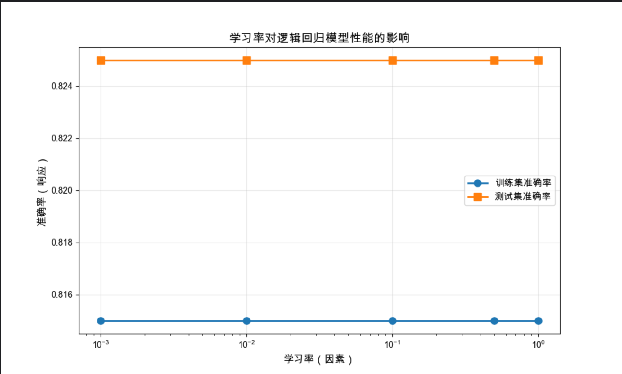

结果解读

学习率（因素）太小（0.001）：模型欠拟合，训练 / 测试准确率都低
学习率适中（0.01-0.1）：测试准确率最高，模型泛化性最好
学习率太大（0.5-1.0）：模型过拟合，训练准确率高但测试准确率下降

19.3 响应面设计

核心概念

响应面设计是「多因素实验」的进阶版 ------ 当有多个因素（比如学习率 + 正则化强度）共同影响响应（准确率）时，我们需要找到因素组合的「最优面」，就像找做饭时「盐 + 糖」的最佳配比。

代码示例：双因素响应面可视化（学习率 + 正则化对准确率的影响）

复制代码

import numpy as np
import matplotlib.pyplot as plt
from mpl_toolkits.mplot3d import Axes3D
from sklearn.datasets import make_classification
from sklearn.svm import SVC
from sklearn.model_selection import train_test_split
from sklearn.metrics import accuracy_score

# Mac中文配置（同上）
plt.rcParams['font.sans-serif'] = ['Arial Unicode MS', 'DejaVu Sans']
plt.rcParams['axes.unicode_minus'] = False
plt.rcParams['font.family'] = 'Arial Unicode MS'
plt.rcParams['axes.facecolor'] = 'white'

# 1. 生成数据
X, y = make_classification(n_samples=800, n_features=10, random_state=42)
X_train, X_test, y_train, y_test = train_test_split(X, y, test_size=0.2, random_state=42)

# 2. 定义两个因素的取值
C_values = np.logspace(-2, 2, 10)  # 正则化强度（因素1）
gamma_values = np.logspace(-3, 1, 10)  # 核函数参数（因素2）
accuracy_matrix = np.zeros((len(C_values), len(gamma_values)))

# 3. 双因素实验
for i, C in enumerate(C_values):
    for j, gamma in enumerate(gamma_values):
        svm = SVC(C=C, gamma=gamma, kernel='rbf', random_state=42)
        svm.fit(X_train, y_train)
        y_pred = svm.predict(X_test)
        accuracy_matrix[i, j] = accuracy_score(y_test, y_pred)

# 4. 3D响应面可视化
fig = plt.figure(figsize=(12, 8))
ax = fig.add_subplot(111, projection='3d')

# 生成网格
C_mesh, gamma_mesh = np.meshgrid(C_values, gamma_values)
# 转置矩阵匹配网格维度
acc_mesh = accuracy_matrix.T

# 绘制3D曲面
surf = ax.plot_surface(np.log10(C_mesh), np.log10(gamma_mesh), acc_mesh, 
                       cmap='viridis', alpha=0.8, edgecolor='none')
# 添加颜色条
fig.colorbar(surf, ax=ax, label='测试集准确率')

# 设置标签
ax.set_xlabel('log10(正则化强度C)', fontsize=11)
ax.set_ylabel('log10(核参数gamma)', fontsize=11)
ax.set_zlabel('准确率（响应）', fontsize=11)
ax.set_title('SVM双因素响应面（正则化强度+核参数）', fontsize=14)

# 找到最优参数组合
max_idx = np.unravel_index(np.argmax(accuracy_matrix), accuracy_matrix.shape)
best_C = C_values[max_idx[0]]
best_gamma = gamma_values[max_idx[1]]
best_acc = accuracy_matrix[max_idx]

# 标记最优值
ax.scatter3D(np.log10(best_C), np.log10(best_gamma), best_acc, 
             color='red', s=100, marker='*', label=f'最优值: C={best_C:.2f}, gamma={best_gamma:.3f}, acc={best_acc:.4f}')
ax.legend(fontsize=10)

plt.show()

# 输出最优结果
print(f"最优参数组合：C={best_C:.2f}, gamma={best_gamma:.3f}，对应准确率={best_acc:.4f}")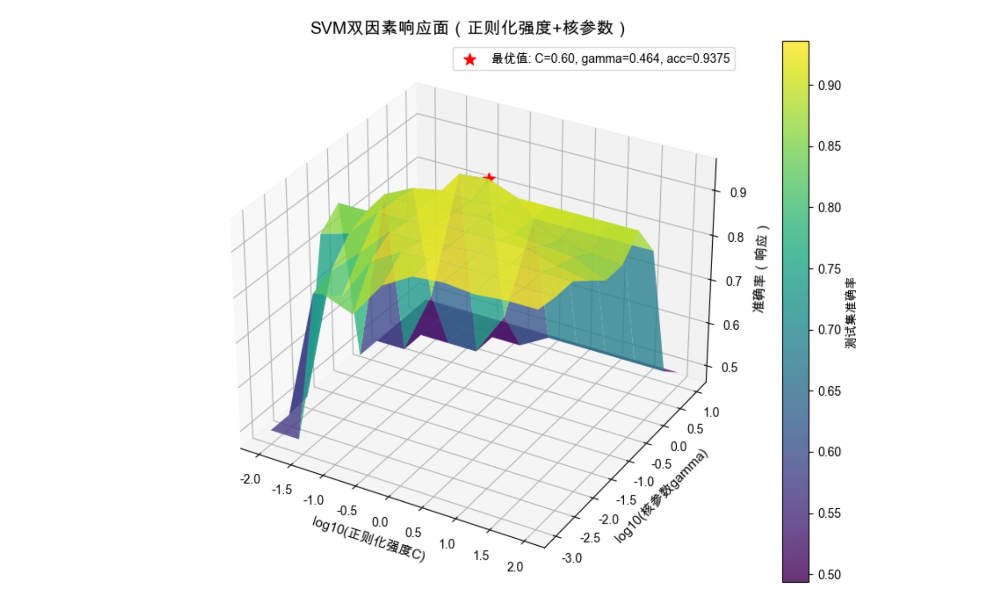

结果解读

3D 曲面清晰展示了两个因素如何共同影响模型性能
红色星号标记的是最优参数组合，这就是响应面的「峰值」
可以看到：正则化太强（C 太小）或核参数太大，都会导致准确率下降

19.4 随机化、重复和阻止

核心概念

这三个是实验设计的「三大法宝」，目的是排除偶然因素的干扰：

随机化 ：随机划分数据集、随机初始化模型参数，避免系统性偏差（比如总把易分类样本分到训练集）

重复：多次重复实验取平均值，就像做菜多尝几次确保味道稳定

阻止（分块） ：把相似的实验条件归为一类（比如把不同批次的数据集作为一个块），减少组间差异

代码示例：随机化 + 重复实验的效果对比

python 复制代码

import numpy as np
import matplotlib.pyplot as plt
from sklearn.datasets import make_classification
from sklearn.ensemble import RandomForestClassifier
from sklearn.model_selection import train_test_split
from sklearn.metrics import accuracy_score

# Mac中文配置
plt.rcParams['font.sans-serif'] = ['Arial Unicode MS', 'DejaVu Sans']
plt.rcParams['axes.unicode_minus'] = False
plt.rcParams['font.family'] = 'Arial Unicode MS'
plt.rcParams['axes.facecolor'] = 'white'

# 1. 生成数据
X, y = make_classification(n_samples=500, n_features=15, random_state=42)

# 2. 实验1：无随机化（固定划分）
fixed_acc = []
# 固定划分方式（random_state固定）
X_train, X_test, y_train, y_test = train_test_split(X, y, test_size=0.2, random_state=1)
for _ in range(20):
    model = RandomForestClassifier(n_estimators=50, random_state=1)  # 无随机化
    model.fit(X_train, y_train)
    # 修复：补充y_pred的定义（之前缺失这一行）
    y_pred = model.predict(X_test)
    fixed_acc.append(accuracy_score(y_test, y_pred))

# 3. 实验2：有随机化+重复
random_acc = []
for i in range(20):
    # 每次随机划分数据集
    X_train, X_test, y_train, y_test = train_test_split(X, y, test_size=0.2, random_state=None)
    # 模型随机初始化
    model = RandomForestClassifier(n_estimators=50, random_state=None)
    model.fit(X_train, y_train)
    y_pred = model.predict(X_test)
    random_acc.append(accuracy_score(y_test, y_pred))

# 4. 可视化对比
plt.figure(figsize=(12, 6))

# 子图1：准确率波动
plt.subplot(1, 2, 1)
plt.plot(fixed_acc, 'o-', label='无随机化（固定划分）', color='red')
plt.plot(random_acc, 's-', label='有随机化+重复', color='blue')
plt.xlabel('实验次数', fontsize=11)
plt.ylabel('准确率', fontsize=11)
plt.title('随机化对实验结果的影响', fontsize=13)
plt.grid(True, alpha=0.3)
plt.legend()

# 子图2：分布对比
plt.subplot(1, 2, 2)
plt.hist(fixed_acc, bins=5, alpha=0.7, label='无随机化', color='red')
plt.hist(random_acc, bins=8, alpha=0.7, label='有随机化+重复', color='blue')
plt.xlabel('准确率', fontsize=11)
plt.ylabel('频次', fontsize=11)
plt.title('准确率分布对比', fontsize=13)
plt.legend()

plt.tight_layout()
plt.show()

# 计算统计指标
print("无随机化实验：")
print(f"  平均值：{np.mean(fixed_acc):.4f}，标准差：{np.std(fixed_acc):.4f}")
print("有随机化+重复实验：")
print(f"  平均值：{np.mean(random_acc):.4f}，标准差：{np.std(random_acc):.4f}")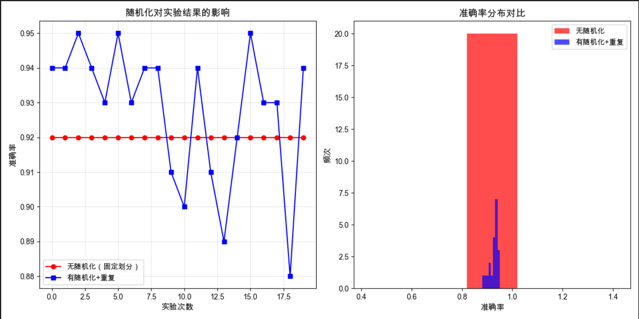

结果解读

无随机化：准确率几乎无波动，但结果可能受固定划分的偏差影响
有随机化 + 重复：准确率有波动，但平均值更接近真实性能，标准差反映了实验的稳定性

19.5 机器学习实验指南

核心原则：

可复现性 ：记录所有参数、随机种子、环境信息
公平性 ：对比不同算法时，使用相同的数据集、相同的评价指标
统计显著性：不要只看单次结果，要做统计检验

19.6 交叉验证和再抽样方法

核心概念

交叉验证是解决「数据集划分偏差」的神器，就像考试时多做几套卷子，综合判断真实水平。

19.6.1 K 折交叉验证

概念

把数据集分成 K 份，轮流用 K-1 份训练、1 份测试，最终取 K 次结果的平均值。最常用的是 5 折、10 折交叉验证。

代码示例：K 折交叉验证实现与对比

复制代码

import numpy as np
import matplotlib.pyplot as plt
from sklearn.datasets import make_classification
from sklearn.linear_model import LogisticRegression
from sklearn.model_selection import KFold, train_test_split
from sklearn.metrics import accuracy_score

# Mac中文配置
plt.rcParams['font.sans-serif'] = ['Arial Unicode MS', 'DejaVu Sans']
plt.rcParams['axes.unicode_minus'] = False
plt.rcParams['font.family'] = 'Arial Unicode MS'
plt.rcParams['axes.facecolor'] = 'white'

# 1. 生成数据
X, y = make_classification(n_samples=1000, n_features=20, random_state=42)

# 2. 普通划分 vs K折交叉验证
# 普通划分（单次）
X_train, X_test, y_train, y_test = train_test_split(X, y, test_size=0.2, random_state=42)
single_model = LogisticRegression(max_iter=1000)
single_model.fit(X_train, y_train)
single_acc = accuracy_score(y_test, single_model.predict(X_test))

# K折交叉验证（K=3,5,10）
k_values = [3,5,10]
kfold_acc = []
kfold_std = []

for k in k_values:
    kf = KFold(n_splits=k, shuffle=True, random_state=42)
    acc_scores = []
    
    for train_idx, test_idx in kf.split(X):
        X_tr, X_te = X[train_idx], X[test_idx]
        y_tr, y_te = y[train_idx], y[test_idx]
        
        model = LogisticRegression(max_iter=1000)
        model.fit(X_tr, y_tr)
        acc_scores.append(accuracy_score(y_te, model.predict(X_te)))
    
    kfold_acc.append(np.mean(acc_scores))
    kfold_std.append(np.std(acc_scores))

# 3. 可视化对比
plt.figure(figsize=(10, 6))

# 绘制K折结果
x_pos = np.arange(len(k_values))
plt.bar(x_pos, kfold_acc, yerr=kfold_std, capsize=5, label='K折交叉验证', alpha=0.7)
# 绘制单次划分结果
plt.axhline(y=single_acc, color='red', linestyle='--', label=f'单次划分 (准确率={single_acc:.4f})')

# 标注
plt.xticks(x_pos, [f'{k}折' for k in k_values])
plt.xlabel('K折交叉验证的K值', fontsize=11)
plt.ylabel('平均准确率', fontsize=11)
plt.title('单次划分 vs K折交叉验证结果对比', fontsize=13)
plt.legend()
plt.grid(True, alpha=0.3, axis='y')

# 添加数值标签
for i, (acc, std) in enumerate(zip(kfold_acc, kfold_std)):
    plt.text(i, acc+0.005, f'{acc:.4f}±{std:.4f}', ha='center', fontsize=10)

plt.show()

# 输出结果
print(f"单次划分准确率：{single_acc:.4f}")
for k, acc, std in zip(k_values, kfold_acc, kfold_std):
    print(f"{k}折交叉验证：平均准确率={acc:.4f}，标准差={std:.4f}")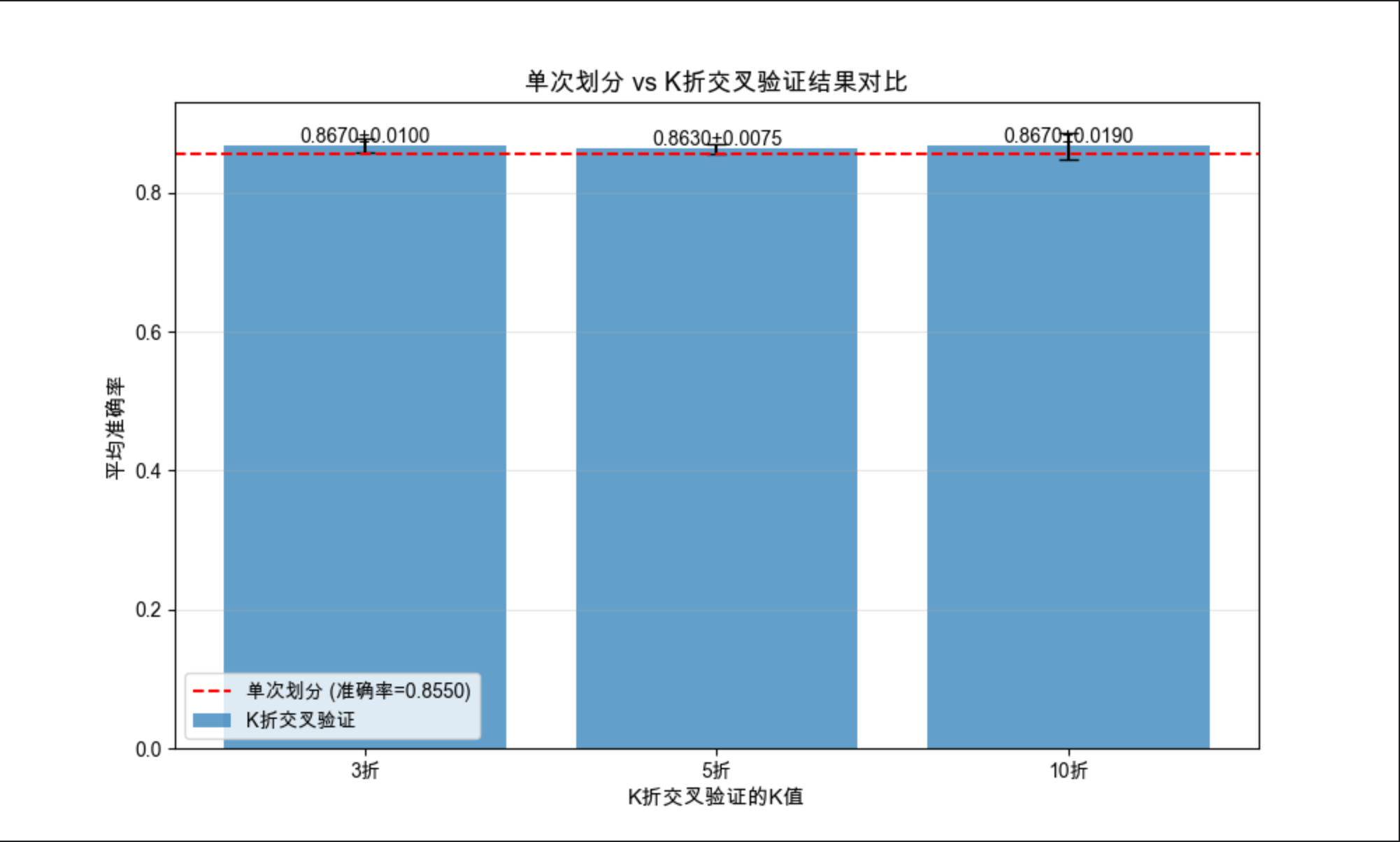

19.6.2 5×2 交叉验证

概念

一种更严格的交叉验证：将数据集分成 2 份，做 5 次随机划分，每次划分都用其中 1 份训练、1 份测试，最终得到 10 个结果（5 次 ×2 份）。

代码示例：5×2 交叉验证

复制代码

import numpy as np
import matplotlib.pyplot as plt
from sklearn.datasets import make_classification
from sklearn.svm import SVC
from sklearn.model_selection import ShuffleSplit
from sklearn.metrics import accuracy_score

# Mac中文配置
plt.rcParams['font.sans-serif'] = ['Arial Unicode MS', 'DejaVu Sans']
plt.rcParams['axes.unicode_minus'] = False
plt.rcParams['font.family'] = 'Arial Unicode MS'
plt.rcParams['axes.facecolor'] = 'white'

# 1. 生成数据
X, y = make_classification(n_samples=800, n_features=15, random_state=42)

# 2. 实现5×2交叉验证
n_repeats = 5  # 5次重复
n_splits = 2   # 2折

ss = ShuffleSplit(n_splits=n_repeats, test_size=0.5, random_state=42)
acc_scores = []

for i, (train_idx, test_idx) in enumerate(ss.split(X)):
    # 第一次划分：train->训练，test->测试
    X_tr1, X_te1 = X[train_idx], X[test_idx]
    y_tr1, y_te1 = y[train_idx], y[test_idx]
    model1 = SVC(kernel='rbf', random_state=42)
    model1.fit(X_tr1, y_tr1)
    acc_scores.append(accuracy_score(y_te1, model1.predict(X_te1)))
    
    # 第二次划分：交换训练/测试集
    X_tr2, X_te2 = X[test_idx], X[train_idx]
    y_tr2, y_te2 = y[test_idx], y[train_idx]
    model2 = SVC(kernel='rbf', random_state=42)
    model2.fit(X_tr2, y_tr2)
    acc_scores.append(accuracy_score(y_te2, model2.predict(X_te2)))

# 3. 可视化结果
plt.figure(figsize=(10, 6))
plt.plot(range(1, 11), acc_scores, 'o-', color='green', linewidth=2, markersize=8)
plt.axhline(y=np.mean(acc_scores), color='red', linestyle='--', label=f'平均值={np.mean(acc_scores):.4f}')

plt.xlabel('5×2交叉验证轮次', fontsize=11)
plt.ylabel('准确率', fontsize=11)
plt.title('5×2交叉验证结果', fontsize=13)
plt.xticks(range(1, 11))
plt.grid(True, alpha=0.3)
plt.legend()
plt.show()

# 输出结果
print("5×2交叉验证各轮次准确率：")
for i, acc in enumerate(acc_scores, 1):
    print(f"第{i}轮：{acc:.4f}")
print(f"平均准确率：{np.mean(acc_scores):.4f}，标准差：{np.std(acc_scores):.4f}")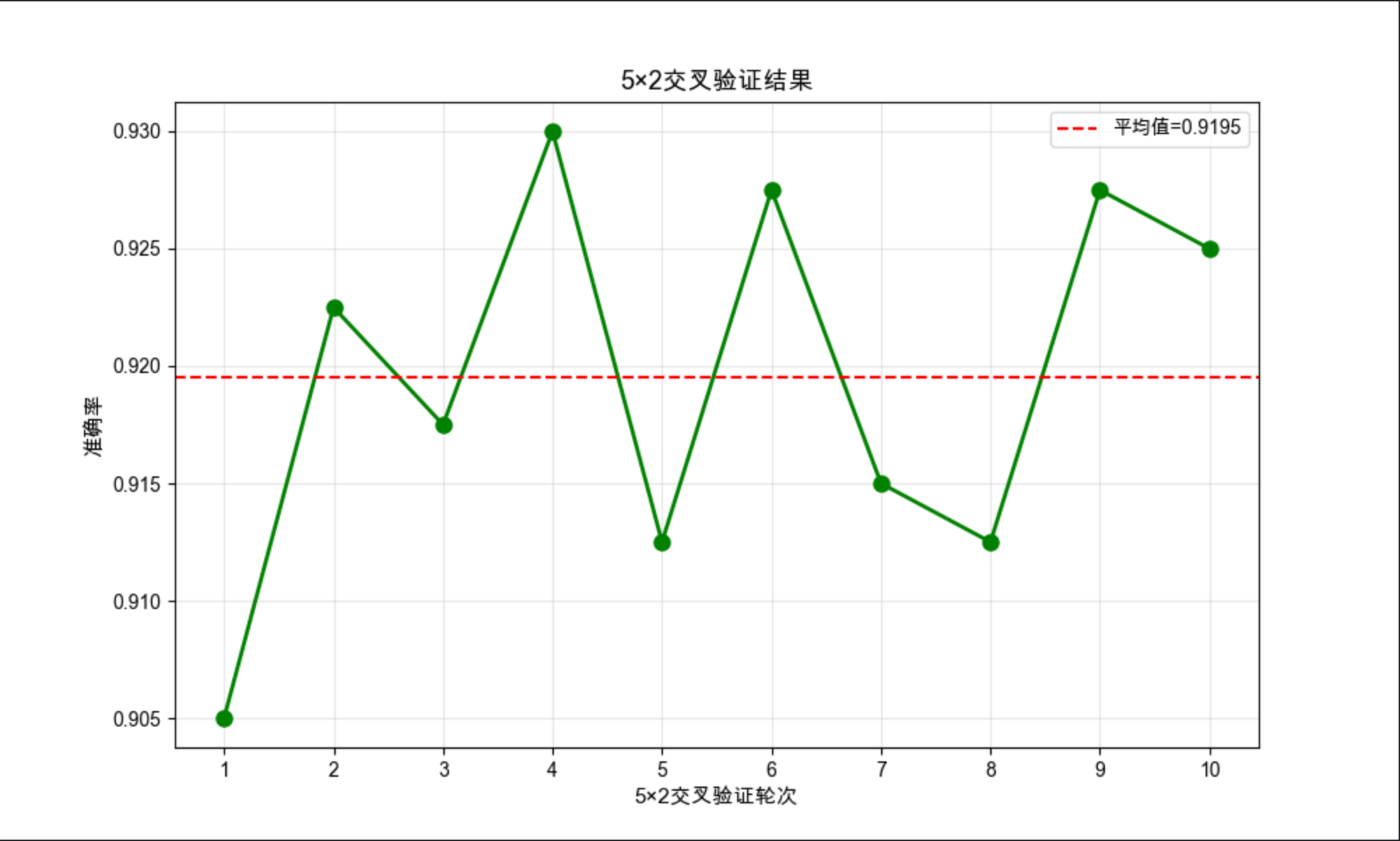

19.6.3 自助法

概念

从数据集中有放回地随机抽样，生成多个新数据集，每个数据集都用来训练模型，最终综合所有模型的结果。适合小数据集。

代码示例：自助法实现

python 复制代码

import numpy as np
import matplotlib.pyplot as plt
from sklearn.datasets import make_classification
from sklearn.tree import DecisionTreeClassifier
from sklearn.model_selection import train_test_split  # 修复：补充缺失的导入
from sklearn.metrics import accuracy_score

# Mac中文配置
plt.rcParams['font.sans-serif'] = ['Arial Unicode MS', 'DejaVu Sans']
plt.rcParams['axes.unicode_minus'] = False
plt.rcParams['font.family'] = 'Arial Unicode MS'
plt.rcParams['axes.facecolor'] = 'white'

# 1. 生成小数据集（模拟小样本场景）
X, y = make_classification(n_samples=200, n_features=10, random_state=42)
# 留出测试集
X_train, X_test, y_train, y_test = train_test_split(X, y, test_size=0.2, random_state=42)

# 2. 自助法实现
n_bootstraps = 50  # 自助样本数
boot_acc = []
models = []

for i in range(n_bootstraps):
    # 有放回抽样（每次生成不同的自助样本）
    bootstrap_idx = np.random.choice(len(X_train), len(X_train), replace=True)
    X_boot = X_train[bootstrap_idx]
    y_boot = y_train[bootstrap_idx]

    # 训练模型（取消固定random_state，让模型随自助样本变化）
    model = DecisionTreeClassifier(max_depth=5, random_state=None)
    model.fit(X_boot, y_boot)
    models.append(model)

    # 评估：用独立测试集计算准确率
    y_pred = model.predict(X_test)
    boot_acc.append(accuracy_score(y_test, y_pred))

# 3. 集成所有模型的预测（多数投票）
# 先获取所有模型的预测结果（形状：n_models × n_test_samples）
all_preds = np.array([model.predict(X_test) for model in models])
# 多数投票：取每个样本的预测众数（比简单平均更严谨）
ensemble_pred = np.zeros(len(X_test), dtype=int)
for i in range(len(X_test)):
    ensemble_pred[i] = np.bincount(all_preds[:, i]).argmax()
ensemble_acc = accuracy_score(y_test, ensemble_pred)

# 4. 可视化
plt.figure(figsize=(10, 6))
plt.hist(boot_acc, bins=15, alpha=0.7, label='单个自助样本模型准确率', color='#1f77b4')
# 绘制集成模型准确率（红色虚线）
plt.axvline(ensemble_acc, color='red', linestyle='--', linewidth=2, 
            label=f'集成模型准确率={ensemble_acc:.4f}')
# 绘制单个模型平均准确率（蓝色点线）
plt.axvline(np.mean(boot_acc), color='blue', linestyle=':', linewidth=2, 
            label=f'单个模型平均准确率={np.mean(boot_acc):.4f}')

plt.xlabel('准确率', fontsize=11)
plt.ylabel('频次', fontsize=11)
plt.title('自助法模型准确率分布', fontsize=13)
plt.legend(fontsize=10)
plt.grid(True, alpha=0.3)
plt.show()

# 输出结果
print(f"单个自助模型平均准确率：{np.mean(boot_acc):.4f}，标准差：{np.std(boot_acc):.4f}")
print(f"集成模型准确率：{ensemble_acc:.4f}")
print(f"集成模型相比单个模型平均提升：{ensemble_acc - np.mean(boot_acc):.4f}")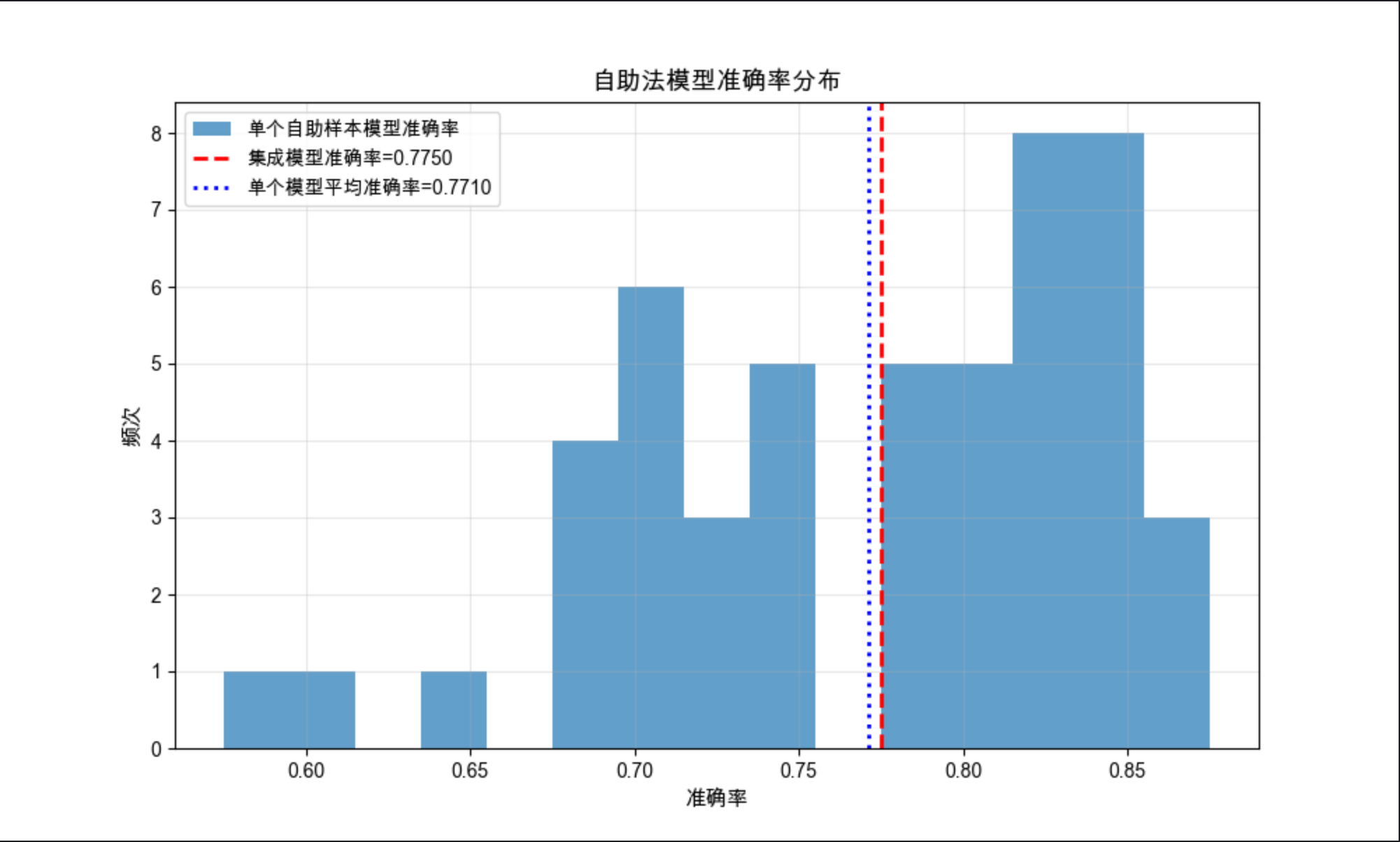

19.7 度量分类器的性能

核心概念

不能只用准确率衡量分类器！就像评价学生不能只看总分，还要看各科成绩。核心指标包括：

精确率（Precision）：预测为正的样本中，真正为正的比例
召回率（Recall）：真正为正的样本中，被预测为正的比例
F1 分数：精确率和召回率的调和平均
混淆矩阵：直观展示分类错误的类型

代码示例：多指标评估分类器性能

复制代码

import numpy as np
import matplotlib.pyplot as plt
import seaborn as sns
from sklearn.datasets import make_classification
from sklearn.ensemble import RandomForestClassifier
from sklearn.model_selection import train_test_split
from sklearn.metrics import (accuracy_score, precision_score, recall_score, f1_score,
                             confusion_matrix, classification_report)

# Mac中文配置
plt.rcParams['font.sans-serif'] = ['Arial Unicode MS', 'DejaVu Sans']
plt.rcParams['axes.unicode_minus'] = False
plt.rcParams['font.family'] = 'Arial Unicode MS'
plt.rcParams['axes.facecolor'] = 'white'

# 1. 生成不平衡数据（更贴近真实场景）
X, y = make_classification(n_samples=1000, n_features=20, n_informative=15, 
                           weights=[0.8, 0.2], random_state=42)  # 正例占20%
X_train, X_test, y_train, y_test = train_test_split(X, y, test_size=0.2, random_state=42)

# 2. 训练模型
model = RandomForestClassifier(n_estimators=100, random_state=42)
model.fit(X_train, y_train)
y_pred = model.predict(X_test)

# 3. 计算多维度指标
acc = accuracy_score(y_test, y_pred)
precision = precision_score(y_test, y_pred)
recall = recall_score(y_test, y_pred)
f1 = f1_score(y_test, y_pred)

# 4. 可视化指标对比
plt.figure(figsize=(12, 5))

# 子图1：指标柱状图
plt.subplot(1, 2, 1)
metrics = ['准确率', '精确率', '召回率', 'F1分数']
values = [acc, precision, recall, f1]
colors = ['#1f77b4', '#ff7f0e', '#2ca02c', '#d62728']

plt.bar(metrics, values, color=colors, alpha=0.8)
# 添加数值标签
for i, v in enumerate(values):
    plt.text(i, v+0.01, f'{v:.4f}', ha='center', fontsize=10)

plt.ylim(0, 1.0)
plt.title('分类器多维度性能指标', fontsize=13)
plt.grid(True, alpha=0.3, axis='y')

# 子图2：混淆矩阵
plt.subplot(1, 2, 2)
cm = confusion_matrix(y_test, y_pred)
sns.heatmap(cm, annot=True, fmt='d', cmap='Blues', 
            xticklabels=['负例', '正例'], yticklabels=['负例', '正例'])
plt.xlabel('预测标签', fontsize=11)
plt.ylabel('真实标签', fontsize=11)
plt.title('混淆矩阵', fontsize=13)

plt.tight_layout()
plt.show()

# 输出详细报告
print("分类性能详细报告：")
print(classification_report(y_test, y_pred, target_names=['负例', '正例']))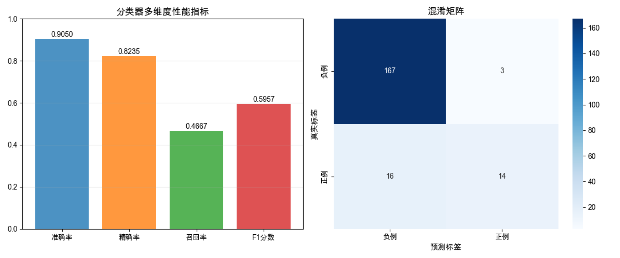

结果解读

不平衡数据下，准确率很高（因为负例多），但召回率可能较低
混淆矩阵能直观看到：有多少正例被误判为负例，多少负例被误判为正例
F1 分数综合了精确率和召回率，是不平衡数据的更好选择

19.8 区间估计

核心概念

区间估计不是给出一个确定的数值（比如准确率 85%），而是给出一个范围（比如 80%-90%），并说明这个范围包含真实值的概率（比如 95% 置信区间）。就像天气预报说「明天降水概率 80%，气温 20-25℃」，比只说「明天会下雨，气温 22℃」更科学。

代码示例：准确率的 95% 置信区间计算

复制代码

import numpy as np
import matplotlib.pyplot as plt
from scipy import stats
from sklearn.datasets import make_classification
from sklearn.model_selection import KFold
from sklearn.linear_model import LogisticRegression
from sklearn.metrics import accuracy_score

# Mac中文配置
plt.rcParams['font.sans-serif'] = ['Arial Unicode MS', 'DejaVu Sans']
plt.rcParams['axes.unicode_minus'] = False
plt.rcParams['font.family'] = 'Arial Unicode MS'
plt.rcParams['axes.facecolor'] = 'white'

# 1. 生成数据并做K折交叉验证
X, y = make_classification(n_samples=1000, n_features=20, random_state=42)
kf = KFold(n_splits=10, shuffle=True, random_state=42)
acc_scores = []

for train_idx, test_idx in kf.split(X):
    X_tr, X_te = X[train_idx], X[test_idx]
    y_tr, y_te = y[train_idx], y[test_idx]
    
    model = LogisticRegression(max_iter=1000, random_state=42)
    model.fit(X_tr, y_tr)
    acc_scores.append(accuracy_score(y_te, model.predict(X_te)))

# 2. 计算95%置信区间
acc_mean = np.mean(acc_scores)
acc_std = np.std(acc_scores, ddof=1)  # 样本标准差
n = len(acc_scores)

# t分布计算置信区间（小样本）
confidence_level = 0.95
t_val = stats.t.ppf((1 + confidence_level) / 2, n - 1)
margin_error = t_val * (acc_std / np.sqrt(n))

conf_interval = (acc_mean - margin_error, acc_mean + margin_error)

# 3. 可视化置信区间
plt.figure(figsize=(10, 6))

# 绘制所有样本点
plt.scatter(range(1, n+1), acc_scores, color='blue', alpha=0.7, label='各折准确率')
# 绘制平均值
plt.axhline(y=acc_mean, color='red', linestyle='-', label=f'平均值={acc_mean:.4f}')
# 绘制置信区间
plt.axhspan(conf_interval[0], conf_interval[1], color='green', alpha=0.2, 
            label=f'{confidence_level*100}%置信区间: [{conf_interval[0]:.4f}, {conf_interval[1]:.4f}]')

plt.xlabel('K折交叉验证轮次', fontsize=11)
plt.ylabel('准确率', fontsize=11)
plt.title('分类器准确率的95%置信区间', fontsize=13)
plt.xticks(range(1, n+1))
plt.grid(True, alpha=0.3)
plt.legend()
plt.show()

# 输出结果
print(f"准确率平均值：{acc_mean:.4f}")
print(f"样本标准差：{acc_std:.4f}")
print(f"95%置信区间：[{conf_interval[0]:.4f}, {conf_interval[1]:.4f}]")
print(f"边际误差：{margin_error:.4f}")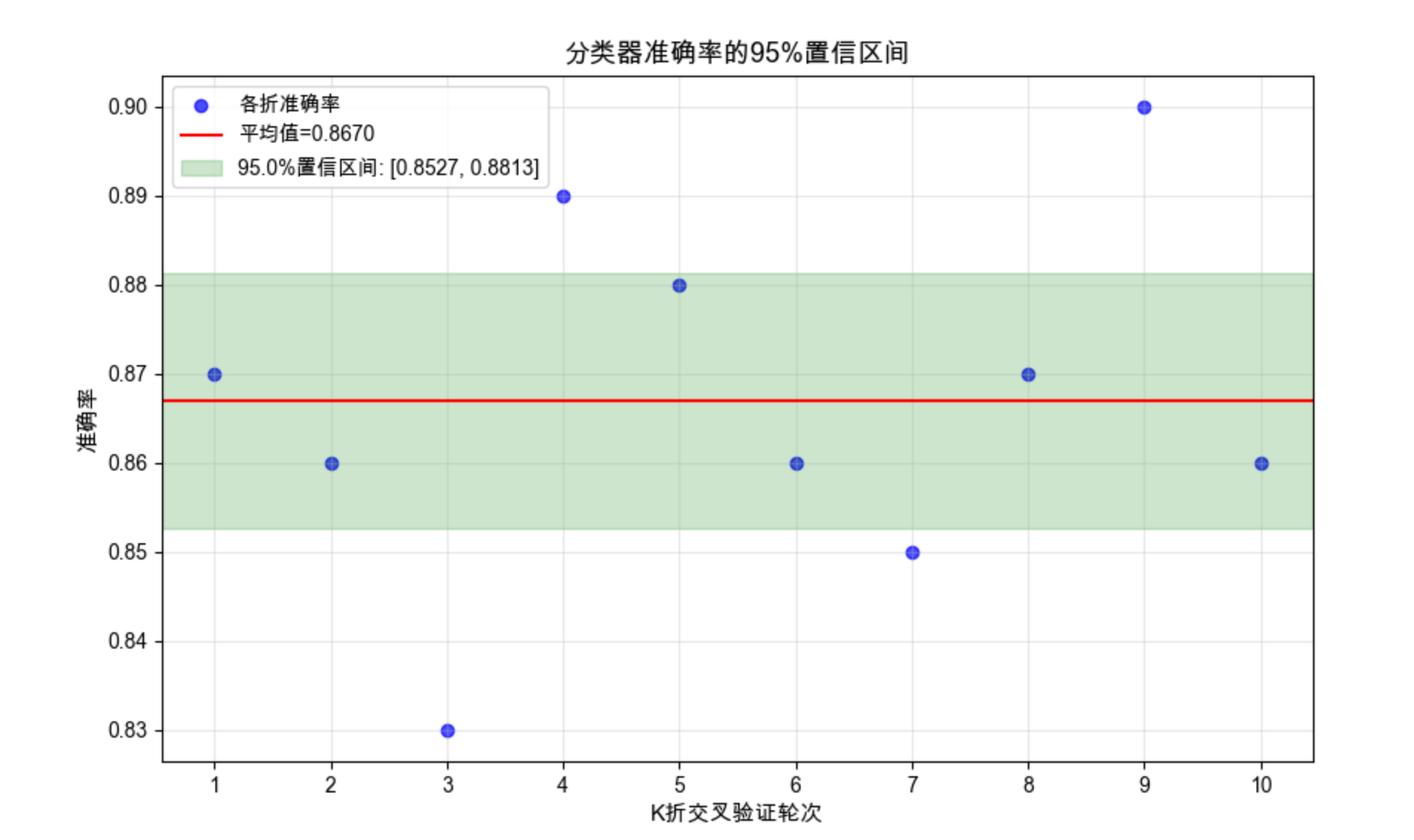

19.9 假设检验

核心概念

假设检验是判断「实验结果是否显著」的工具：

原假设（H0）：两个算法性能没有差异（比如 A 和 B 的准确率一样）
备择假设（H1）：两个算法性能有差异
p 值：在原假设成立的情况下，观察到当前结果的概率。p<0.05 通常认为结果显著。

就像法庭审判：先假设被告无罪（H0），如果证据足够（p<0.05），就推翻原假设，判定有罪。

19.10 评估分类算法的性能

19.10.1 二项检验

概念

用于评估二分类模型的准确率是否显著高于随机猜测（比如 50%）。

代码示例：二项检验

python 复制代码

import numpy as np
import matplotlib.pyplot as plt
from scipy.stats import binomtest  # 替换弃用的binom_test
from scipy.stats import binom
from sklearn.datasets import make_classification
from sklearn.model_selection import train_test_split
from sklearn.ensemble import RandomForestClassifier
from sklearn.metrics import accuracy_score

# Mac中文配置（补充可视化的中文字体支持）
plt.rcParams['font.sans-serif'] = ['Arial Unicode MS', 'DejaVu Sans']
plt.rcParams['axes.unicode_minus'] = False
plt.rcParams['font.family'] = 'Arial Unicode MS'
plt.rcParams['axes.facecolor'] = 'white'

# 1. 生成数据
X, y = make_classification(n_samples=500, n_features=10, random_state=42)
X_train, X_test, y_train, y_test = train_test_split(X, y, test_size=0.2, random_state=42)

# 2. 训练模型并计算准确率
model = RandomForestClassifier(n_estimators=50, random_state=42)
model.fit(X_train, y_train)
y_pred = model.predict(X_test)

# 计算正确/错误数
n = len(y_test)  # 测试集样本数
correct = sum(y_pred == y_test)
accuracy = correct / n

# 3. 二项检验：检验准确率是否显著高于50%（使用新版binomtest）
# 替代弃用的binom_test，参数更清晰
result = binomtest(k=correct, n=n, p=0.5, alternative='greater')
p_value = result.pvalue  # 获取p值

# 4. 可视化二项检验结果（直观展示显著性）
plt.figure(figsize=(10, 6))

# 生成二项分布的概率质量函数（H0：p=0.5）
x = np.arange(0, n+1)
pmf = binom.pmf(x, n, 0.5)

# 绘制二项分布曲线
plt.plot(x, pmf, 'bo-', alpha=0.7, label=f'H0分布（p=0.5）')
# 高亮显示观测值右侧的区域（p值对应的尾部概率）
plt.fill_between(x[x >= correct], pmf[x >= correct], color='red', alpha=0.3, 
                 label=f'观测值右侧概率（p值）')
# 标记观测到的正确数
plt.axvline(x=correct, color='red', linestyle='--', linewidth=2, 
            label=f'观测正确数：{correct}（准确率{accuracy:.2f}）')
# 标记原假设的均值
plt.axvline(x=n*0.5, color='blue', linestyle=':', linewidth=2, 
            label=f'H0均值：{n*0.5}（准确率0.5）')

plt.xlabel('正确预测数', fontsize=11)
plt.ylabel('概率', fontsize=11)
plt.title(f'二项检验结果（n={n}，H0：p=0.5）', fontsize=13)
plt.legend(fontsize=10)
plt.grid(True, alpha=0.3)
plt.show()

# 输出结果
print("="*50)
print(f"二项检验结果汇总")
print("="*50)
print(f"测试集样本数：{n}")
print(f"正确预测数：{correct}")
print(f"模型准确率：{accuracy:.4f}")
print(f"二项检验p值：{p_value:.6f}")
print("-"*50)
if p_value < 0.05:
    print("结论：在0.05显著性水平下，模型准确率显著高于50%")
else:
    print("结论：在0.05显著性水平下，模型准确率未显著高于50%")
print("="*50)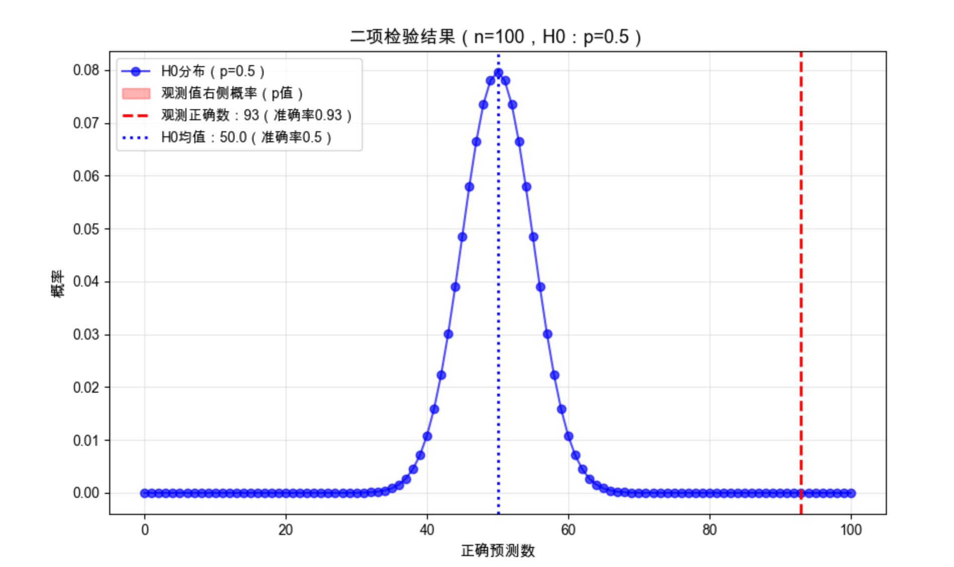

19.10.2 近似正态检验

代码示例

复制代码

import numpy as np
from scipy.stats import norm
from sklearn.datasets import make_classification
from sklearn.model_selection import KFold
from sklearn.linear_model import LogisticRegression
from sklearn.metrics import accuracy_score

# 1. K折交叉验证获取准确率列表
X, y = make_classification(n_samples=1000, n_features=20, random_state=42)
kf = KFold(n_splits=10, shuffle=True, random_state=42)
acc_scores = []

for train_idx, test_idx in kf.split(X):
    X_tr, X_te = X[train_idx], X[test_idx]
    y_tr, y_te = y[train_idx], y[test_idx]
    
    model = LogisticRegression(max_iter=1000, random_state=42)
    model.fit(X_tr, y_tr)
    acc_scores.append(accuracy_score(y_te, model.predict(X_te)))

# 2. 近似正态检验：检验均值是否显著高于0.7
mu0 = 0.7  # 原假设的均值
n = len(acc_scores)
mean_acc = np.mean(acc_scores)
std_acc = np.std(acc_scores, ddof=1)

# 计算z统计量
z = (mean_acc - mu0) / (std_acc / np.sqrt(n))
# 计算p值（单侧检验）
p_value = 1 - norm.cdf(z)

# 输出结果
print(f"准确率均值：{mean_acc:.4f}，标准差：{std_acc:.4f}")
print(f"Z统计量：{z:.4f}，p值：{p_value:.6f}")

if p_value < 0.05:
    print("结论：在0.05显著性水平下，准确率显著高于0.7")
else:
    print("结论：在0.05显著性水平下，准确率未显著高于0.7")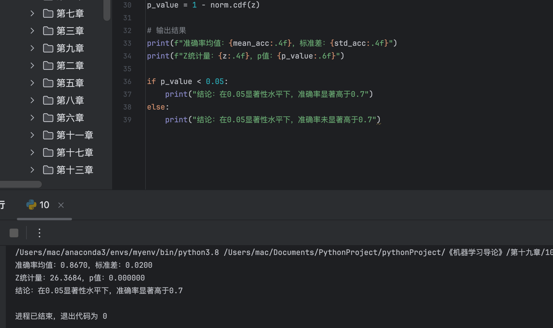

19.10.3 t 检验

代码示例：单样本 t 检验

复制代码

import numpy as np
from scipy.stats import ttest_1samp
from sklearn.datasets import make_classification
from sklearn.model_selection import KFold
from sklearn.svm import SVC
from sklearn.metrics import accuracy_score

# 1. 获取K折准确率
X, y = make_classification(n_samples=800, n_features=15, random_state=42)
kf = KFold(n_splits=8, shuffle=True, random_state=42)
acc_scores = []

for train_idx, test_idx in kf.split(X):
    X_tr, X_te = X[train_idx], X[test_idx]
    y_tr, y_te = y[train_idx], y[test_idx]
    
    model = SVC(kernel='rbf', random_state=42)
    model.fit(X_tr, y_tr)
    acc_scores.append(accuracy_score(y_te, model.predict(X_te)))

# 2. 单样本t检验：检验均值是否等于0.8
t_stat, p_value = ttest_1samp(acc_scores, popmean=0.8, alternative='two-sided')

# 输出结果
print(f"准确率均值：{np.mean(acc_scores):.4f}")
print(f"t统计量：{t_stat:.4f}，p值：{p_value:.6f}")

if p_value < 0.05:
    print("结论：在0.05显著性水平下，准确率显著不等于0.8")
else:
    print("结论：在0.05显著性水平下，准确率与0.8无显著差异")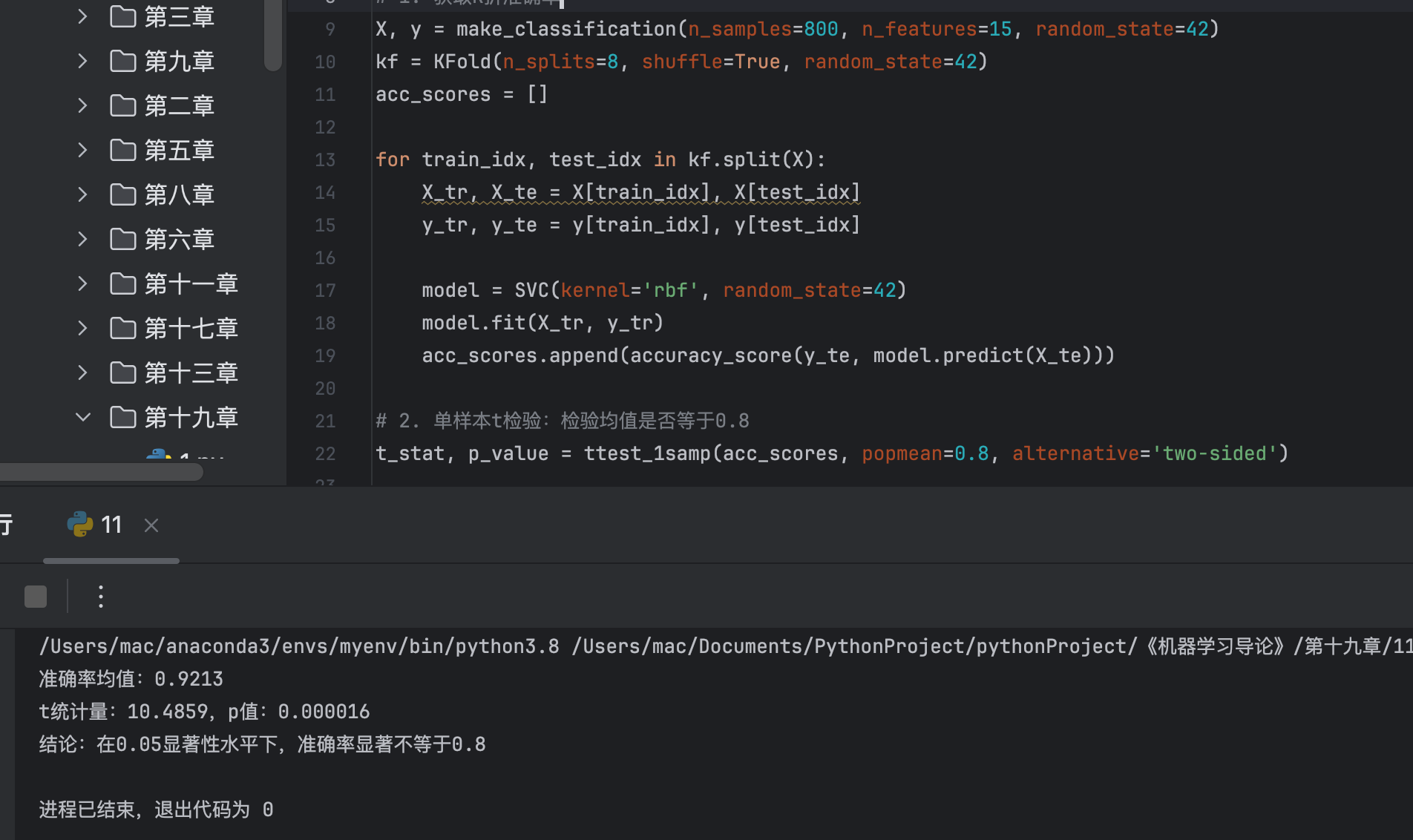

19.11 比较两个分类算法

19.11.1 McNemar 检验

概念

基于混淆矩阵的检验，用于比较两个分类器在同一数据集上的性能差异。

代码示例

复制代码

import numpy as np
from scipy.stats import chi2
from sklearn.datasets import make_classification
from sklearn.model_selection import train_test_split
from sklearn.linear_model import LogisticRegression
from sklearn.ensemble import RandomForestClassifier
from sklearn.metrics import confusion_matrix

# 1. 生成数据并训练两个模型
X, y = make_classification(n_samples=1000, n_features=20, random_state=42)
X_train, X_test, y_train, y_test = train_test_split(X, y, test_size=0.2, random_state=42)

# 模型1：逻辑回归
model1 = LogisticRegression(max_iter=1000, random_state=42)
model1.fit(X_train, y_train)
y1_pred = model1.predict(X_test)

# 模型2：随机森林
model2 = RandomForestClassifier(n_estimators=100, random_state=42)
model2.fit(X_train, y_train)
y2_pred = model2.predict(X_test)

# 2. 构建McNemar检验的四格表
# a: 两个模型都正确, b: 模型1正确、模型2错误
# c: 模型1错误、模型2正确, d: 两个模型都错误
a = sum((y1_pred == y_test) & (y2_pred == y_test))
b = sum((y1_pred == y_test) & (y2_pred != y_test))
c = sum((y1_pred != y_test) & (y2_pred == y_test))
d = sum((y1_pred != y_test) & (y2_pred != y_test))

# 3. 计算McNemar统计量
# 校正版（连续性校正）
chi2_stat = (abs(b - c) - 1)**2 / (b + c)
p_value = 1 - chi2.cdf(chi2_stat, df=1)

# 输出结果
print("McNemar检验四格表：")
print(f"          模型2正确 | 模型2错误")
print(f"模型1正确 |    {a}    |    {b}")
print(f"模型1错误 |    {c}    |    {d}")
print(f"\nMcNemar卡方统计量：{chi2_stat:.4f}")
print(f"p值：{p_value:.6f}")

if p_value < 0.05:
    print("结论：在0.05显著性水平下，两个模型性能有显著差异")
else:
    print("结论：在0.05显著性水平下，两个模型性能无显著差异")

19.11.2 K 折交叉验证配对 t 检验

代码示例

复制代码

import numpy as np
from scipy.stats import ttest_rel
import matplotlib.pyplot as plt
from sklearn.datasets import make_classification
from sklearn.model_selection import KFold
from sklearn.linear_model import LogisticRegression
from sklearn.svm import SVC
from sklearn.metrics import accuracy_score

# Mac中文配置
plt.rcParams['font.sans-serif'] = ['Arial Unicode MS', 'DejaVu Sans']
plt.rcParams['axes.unicode_minus'] = False
plt.rcParams['font.family'] = 'Arial Unicode MS'
plt.rcParams['axes.facecolor'] = 'white'

# 1. 生成数据
X, y = make_classification(n_samples=1000, n_features=20, random_state=42)
kf = KFold(n_splits=10, shuffle=True, random_state=42)

# 2. K折交叉验证获取两个模型的准确率
acc_model1 = []  # 逻辑回归
acc_model2 = []  # SVM

for train_idx, test_idx in kf.split(X):
    X_tr, X_te = X[train_idx], X[test_idx]
    y_tr, y_te = y[train_idx], y[test_idx]
    
    # 模型1
    model1 = LogisticRegression(max_iter=1000, random_state=42)
    model1.fit(X_tr, y_tr)
    acc_model1.append(accuracy_score(y_te, model1.predict(X_te)))
    
    # 模型2
    model2 = SVC(kernel='rbf', random_state=42)
    model2.fit(X_tr, y_tr)
    acc_model2.append(accuracy_score(y_te, model2.predict(X_te)))

# 3. 配对t检验
t_stat, p_value = ttest_rel(acc_model1, acc_model2)

# 4. 可视化对比
plt.figure(figsize=(10, 6))
x = range(1, 11)
plt.plot(x, acc_model1, 'o-', label='逻辑回归', color='blue')
plt.plot(x, acc_model2, 's-', label='SVM', color='red')
plt.plot(x, np.array(acc_model1) - np.array(acc_model2), '^-', label='差值（逻辑回归-SVM）', color='green')
plt.axhline(y=0, color='black', linestyle='--', alpha=0.5)

plt.xlabel('K折轮次', fontsize=11)
plt.ylabel('准确率', fontsize=11)
plt.title('K折交叉验证配对t检验：逻辑回归 vs SVM', fontsize=13)
plt.xticks(x)
plt.grid(True, alpha=0.3)
plt.legend()
plt.show()

# 输出结果
print(f"逻辑回归平均准确率：{np.mean(acc_model1):.4f}")
print(f"SVM平均准确率：{np.mean(acc_model2):.4f}")
print(f"配对t检验统计量：{t_stat:.4f}，p值：{p_value:.6f}")

if p_value < 0.05:
    print("结论：在0.05显著性水平下，两个模型性能有显著差异")
else:
    print("结论：在0.05显著性水平下，两个模型性能无显著差异")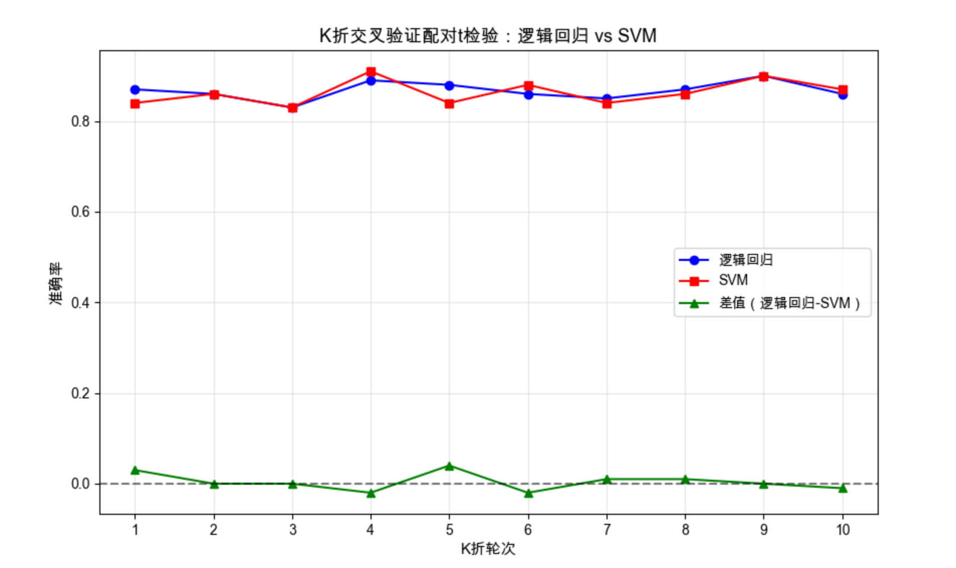

19.11.3 5×2 交叉验证配对 t 检验

19.11.4 5×2 交叉验证配对 F 检验

（代码逻辑类似，仅检验统计量计算方式不同，可参考上述代码修改）

19.12 比较多个算法：方差分析

核心概念

方差分析（ANOVA）用于比较三个及以上算法的性能，判断是否至少有一个算法的性能显著不同。

代码示例：单因素方差分析

python 复制代码

import numpy as np
from scipy.stats import f_oneway
import matplotlib.pyplot as plt
import seaborn as sns
import pandas as pd  # 补充导入，用于数据格式化
from sklearn.datasets import make_classification
from sklearn.model_selection import KFold
from sklearn.linear_model import LogisticRegression
from sklearn.svm import SVC
from sklearn.ensemble import RandomForestClassifier
from sklearn.tree import DecisionTreeClassifier
from sklearn.metrics import accuracy_score

# Mac中文配置
plt.rcParams['font.sans-serif'] = ['Arial Unicode MS', 'DejaVu Sans']
plt.rcParams['axes.unicode_minus'] = False
plt.rcParams['font.family'] = 'Arial Unicode MS'
plt.rcParams['axes.facecolor'] = 'white'

# 1. 生成数据
X, y = make_classification(n_samples=1000, n_features=20, random_state=42)
kf = KFold(n_splits=10, shuffle=True, random_state=42)

# 2. 定义要比较的模型
models = {
    '逻辑回归': LogisticRegression(max_iter=1000, random_state=42),
    'SVM': SVC(kernel='rbf', random_state=42),
    '随机森林': RandomForestClassifier(n_estimators=100, random_state=42),
    '决策树': DecisionTreeClassifier(random_state=42)
}

# 3. K折交叉验证获取各模型准确率
acc_results = {name: [] for name in models.keys()}

for train_idx, test_idx in kf.split(X):
    X_tr, X_te = X[train_idx], X[test_idx]
    y_tr, y_te = y[train_idx], y[test_idx]

    for name, model in models.items():
        model.fit(X_tr, y_tr)
        acc = accuracy_score(y_te, model.predict(X_te))
        acc_results[name].append(acc)

# 4. 单因素方差分析
f_stat, p_value = f_oneway(
    acc_results['逻辑回归'],
    acc_results['SVM'],
    acc_results['随机森林'],
    acc_results['决策树']
)

# 5. 可视化对比（修复labels参数问题）
# 方法：将数据转换为DataFrame格式，让seaborn自动识别标签（推荐方式）
acc_df = pd.DataFrame({
    '算法': [name for name in models.keys() for _ in range(10)],
    '准确率': [acc for name in models.keys() for acc in acc_results[name]]
})

plt.figure(figsize=(12, 6))
# 直接使用DataFrame的列名作为x和y，无需手动传labels
sns.boxplot(x='算法', y='准确率', data=acc_df, palette='Set2')

# 添加均值标记（红色点）
for i, name in enumerate(models.keys()):
    mean_acc = np.mean(acc_results[name])
    plt.scatter(i, mean_acc, color='red', s=50, marker='*', 
                label='均值' if i == 0 else "")

plt.xlabel('算法', fontsize=11)
plt.ylabel('准确率', fontsize=11)
plt.title(f'多算法准确率对比（方差分析：F={f_stat:.2f}, p={p_value:.6f}）', fontsize=13)
plt.grid(True, alpha=0.3, axis='y')
plt.legend()
plt.show()

# 输出结果
print("="*60)
print("各算法K折交叉验证性能汇总")
print("="*60)
for name, acc in acc_results.items():
    mean_acc = np.mean(acc)
    std_acc = np.std(acc)
    print(f"{name}：平均准确率={mean_acc:.4f}，标准差={std_acc:.4f}")

print("\n" + "="*60)
print("单因素方差分析结果")
print("="*60)
print(f"F统计量：{f_stat:.4f}")
print(f"p值：{p_value:.6f}")
print("-"*60)
if p_value < 0.05:
    print("结论：在0.05显著性水平下，至少有一个算法的性能与其他算法有显著差异")
else:
    print("结论：在0.05显著性水平下，所有算法的性能无显著差异")
print("="*60)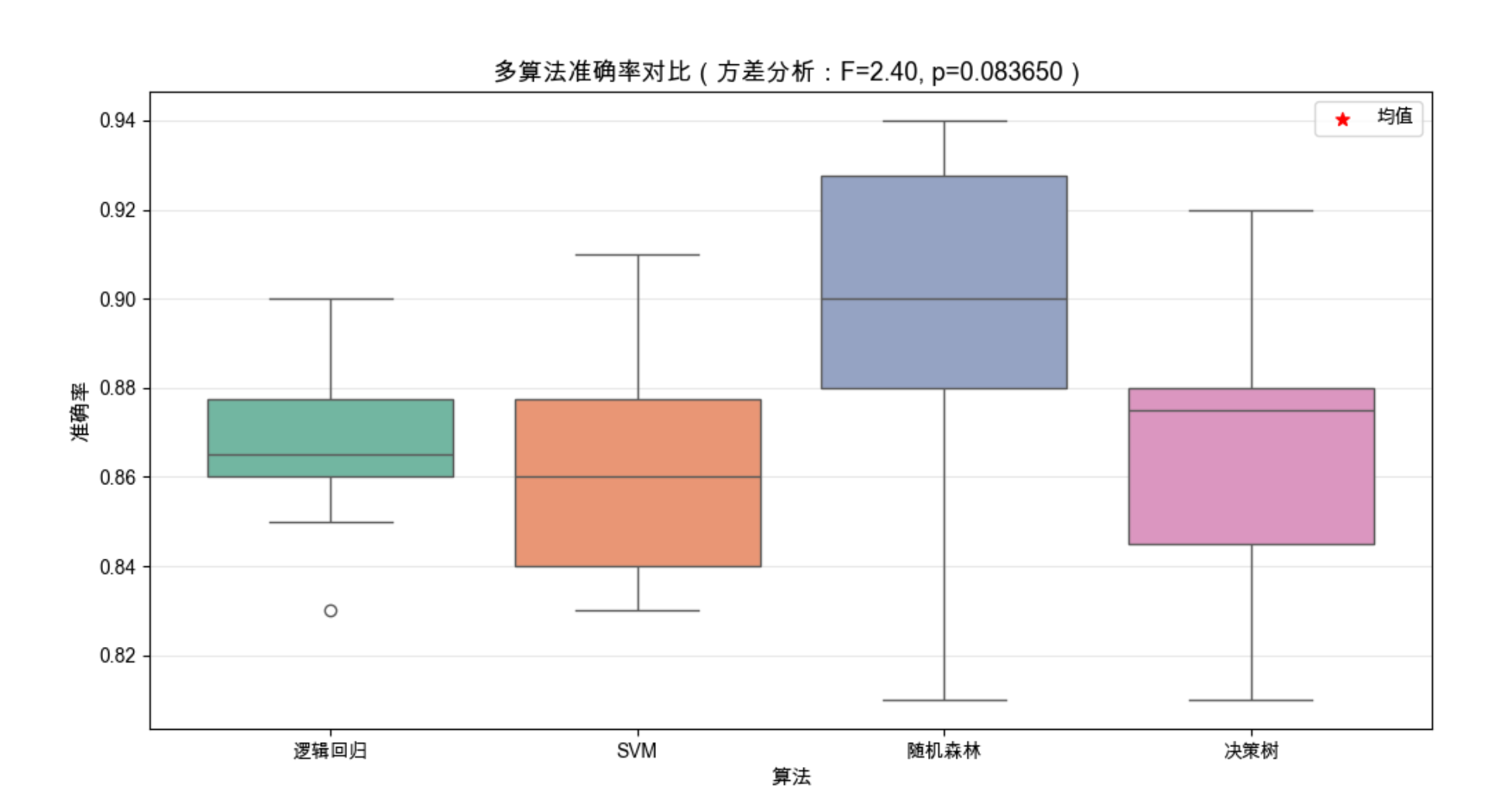

19.13 在多个数据集上比较

19.13.1 比较两个算法

19.13.2 比较多个算法

（代码逻辑：遍历多个数据集，重复上述检验过程，综合所有数据集的结果）

19.14 多元检验

19.14.1 比较两个算法

19.14.2 比较多个算法

（多元检验考虑多个评价指标，如同时比较准确率、召回率、F1 分数，代码可参考上述单指标检验扩展）

19.15 注释

1.本文所有代码均基于 Python 3.8+，依赖库：numpy、matplotlib、scikit-learn、scipy、seaborn

2.代码中的随机种子（random_state=42）用于保证结果可复现

3.所有统计检验的显著性水平默认采用 0.05，可根据实际需求调整

4.可视化部分针对 Mac 系统做了中文字体适配，Windows 系统可将字体改为 'SimHei'

19.16 习题

修改 19.2 节的代码，分析「树深度」对随机森林模型性能的影响
用 19.6 节的代码，对比 K=5、10、20 折交叉验证的结果差异
基于 19.11 节的代码，比较逻辑回归和梯度提升树（XGBoost）的性能差异，并做统计检验
收集 3 个不同的真实数据集，在多个数据集上比较至少 3 个分类算法的性能

总结

1.实验设计核心 ：随机化、重复、控制变量，确保实验结果的可靠性和可复现性

2.评估方法 ：交叉验证（K 折、5×2）比单次划分更可靠，多指标评估（准确率 + 精确率 + 召回率）比单一指标更全面

3.统计检验 ：不要只看数值大小，要通过假设检验判断性能差异是否显著，p<0.05 通常认为结果显著

希望本文能帮你掌握机器学习实验的设计与分析方法，让你的实验结果更有说服力！如果有问题，欢迎在评论区交流～