前言
- 前几天在看论文,打算复现,论文用到了LSTM,故这一篇文章是小编学LSTM模型的学习笔记;
- LSTM感觉很复杂,但是结合代码构建神经网络,又感觉还行;
- 本次学习的案例数据来源于GitHub,在本文案例前有数据和本人代码文件的网盘链接,想学习的可以下载,当然也希望大家能够批评指针,一起学习。
文章目录
1、LSTM讲解
由于本人现在没有学RNN模型,故学习LSTM只聚焦于两个模块:
LSTM的三种类型门:输入门、遗忘门、输出门;LSTM的隐藏层包含"隐状态"和"记忆元",只有隐状态会传递到输出层,而记忆元完全属于内部信息;至于LSTM可以缓解梯度消失和梯度爆炸,就等后面学到RNN之后在详细学习。
1、网络结构
LSTM神经网络简图(用ppt太难画了)
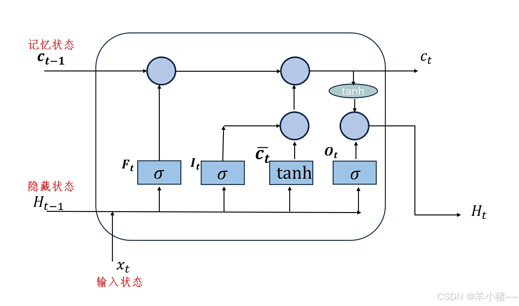
- C:记忆细胞,Ct-1,上一个记忆状态,Ct当下记忆状态
- H:隐藏状态
2、解释
-
遗忘门(Forget Gate):
- 对输入信息x,进行遗忘,选择需要记忆的东西,假如:我们考完了高数,选择需要备考线性代数,这个时候当我们进入这个门时候,需要选择遗忘高数内容(虽然现实不可能)。
f t = σ ( W f ⋅ h t − 1 , x t + b f ) f_t=\sigma(W_f\cdoth_{t-1},x_t+b_f) ft=σ(Wf⋅ht−1,xt+bf)
- 其中,Wf是权重矩阵,bf是偏置项,σ是 Sigmoid 激活函数,用于决定丢弃多少前一个单元状态的信息。
-
输入门(Input Gate):
- It,选择记忆,假如:我们复习线性代数的时候,可能有些知识是不需要记忆的,而这门的作用就是这个,过滤掉没有用的知识。
i t = σ ( W i ⋅ h t − 1 , x t + b i ) c ~ t = tanh ( W c ⋅ h t − 1 , x t + b c ) i_t=\sigma(W_i\cdoth_{t-1},x_t+b_i)\\\tilde{c}_t=\tanh(W_c\cdoth_{t-1},x_t+b_c) it=σ(Wi⋅ht−1,xt+bi)c~t=tanh(Wc⋅ht−1,xt+bc)
- 其中,Wi和 Wc是权重矩阵,bi和 bc*是偏置项,σ 是 Sigmoid 激活函数,tanh是双曲正切激活函数,用于生成候选单元状态。
-
单元状态(Cell State):
- 这个时候,我们记忆力多少呢?这个门相当于我们复习完一次在脑子里还剩下多少知识。
c t = f t ⊙ c t − 1 + i t ⊙ c ~ t c_t=f_t\odot c_{t-1}+i_t\odot\tilde{c}_t ct=ft⊙ct−1+it⊙c~t
- 其中,⊙是逐元素乘法(Hadamard product),用于更新单元状态。
-
输出门(Output Gate):
- 输出隐藏维度,相当于我们考试成绩,在神经网络中,它相当于输出多少维度特征
o t = σ ( W o ⋅ h t − 1 , x t + b o ) h t = o t ⊙ tanh ( c t ) o_t=\sigma(W_o\cdoth_{t-1},x_t+b_o)\\h_t=o_t\odot\tanh(c_t) ot=σ(Wo⋅ht−1,xt+bo)ht=ot⊙tanh(ct)
- 其中,Wo 是权重矩阵,bo 是偏置项,σ 是 Sigmoid 激活函数,tanh是双曲正切激活函数,用于生成当前时间步的隐藏状态。
3、前言
当然 ,结合案例实战,看代码是如何构建神经网络的才是最重要的,下面就是一个股价预测案例,核心是在于怎么构建LSTM网络结构,怎么进行前向传播
2、案例
数据来源于GitHub,数据和本人代码的文件网盘下载如下:
通过网盘分享的文件:基于LSTM的股价预测(入门).zip
链接: https://pan.baidu.com/s/1ZXFLl_TrhReexyvb5Gp8Xg?pwd=v7t2 提取码: v7t2
1、数据分析
1、导入库
python
# 导入常用的库
import numpy as np
import pandas as pd
import matplotlib.pyplot as plt
import torch
import torch.nn as nn
# 显示中文
from pylab import mpl
mpl.rcParams["font.sans-serif"] = ["SimHei"]  # 显示中文
plt.rcParams['axes.unicode_minus'] = False		# 显示负号
2、导入数据
python
dates = pd.date_range('2008-08-25', '2017-10-11', freq='B')
df_main = pd.DataFrame(index=dates)
df_aaxj = pd.read_csv("./data_stock/ETFs/aaxj.us.txt", parse_dates=True, index_col=0) # 索引列为 0
df_main = df_main.join(df_aaxj)   # 按照索引列规定数据范围
df_main
| | Open | High | Low | Close | Volume | OpenInt |
| 2008-08-25 | 44.044 | 44.044 | 43.248 | 43.248 | 18975.0 | 0.0 |
| 2008-08-26 | 43.802 | 43.802 | 43.471 | 43.660 | 5507.0 | 0.0 |
| 2008-08-27 | 44.564 | 44.564 | 44.457 | 44.457 | 1675.0 | 0.0 |
| 2008-08-28 | 44.421 | 44.475 | 44.421 | 44.475 | 6687.0 | 0.0 |
| 2008-08-29 | 44.224 | 44.224 | 44.171 | 44.171 | 446.0 | 0.0 |
| ... | ... | ... | ... | ... | ... | ... |
| 2017-10-05 | 73.500 | 74.030 | 73.500 | 73.970 | 2134323.0 | 0.0 |
| 2017-10-06 | 73.470 | 73.650 | 73.220 | 73.579 | 2092100.0 | 0.0 |
| 2017-10-09 | 73.500 | 73.795 | 73.480 | 73.770 | 879600.0 | 0.0 |
| 2017-10-10 | 74.150 | 74.490 | 74.150 | 74.480 | 1878845.0 | 0.0 |
| 2017-10-11 | 74.290 | 74.645 | 74.210 | 74.610 | 1168511.0 | 0.0 |
|---|
2383 rows × 6 columns
3、数据预处理
python
# 查看数据类型
df_main.info()<class 'pandas.core.frame.DataFrame'>
DatetimeIndex: 2383 entries, 2008-08-25 to 2017-10-11
Freq: B
Data columns (total 6 columns):
# Column Non-Null Count Dtype
--- ------ -------------- -----
0 Open 2298 non-null float64
1 High 2298 non-null float64
2 Low 2298 non-null float64
3 Close 2298 non-null float64
4 Volume 2298 non-null float64
5 OpenInt 2298 non-null float64
dtypes: float64(6)
memory usage: 194.9 KB- 总数量:2383,no_null数量:2298,存在缺失值
- 数据类型:float64
python
# 查看缺失值数量
df_main.isnull().sum()
输出:
Open       85
High       85
Low        85
Close      85
Volume     85
OpenInt    85
dtype: int64- 85 / 2385 大概为3.5%,缺失值有点多;
- 缺失值类型为随机丢失值,是收集缺失的;
- 由于该数据是时间序列,且股票价格和前后关系很大,故采用插值方法填充。
python
# 插值方法填充缺失值
df_main = df_main.interpolate(method='linear')
python
# 再次查看缺失值的情况
df_main.isnull().sum()
输出:
Open       0
High       0
Low        0
Close      0
Volume     0
OpenInt    0
dtype: int64
python
# 统计量分析
df_main.describe()
输出:
| | Open | High | Low | Close | Volume | OpenInt |
| count | 2383.000000 | 2383.000000 | 2383.000000 | 2383.000000 | 2.383000e+03 | 2383.0 |
| mean | 52.559695 | 52.835654 | 52.216654 | 52.552454 | 7.177284e+05 | 0.0 |
| std | 8.773809 | 8.687520 | 8.930144 | 8.805241 | 7.704731e+05 | 0.0 |
| min | 23.790000 | 24.605000 | 19.699000 | 22.726000 | 1.120000e+02 | 0.0 |
| 25% | 48.988500 | 49.313000 | 48.552500 | 48.981500 | 2.789905e+05 | 0.0 |
| 50% | 53.653000 | 53.932000 | 53.432000 | 53.653000 | 5.040570e+05 | 0.0 |
| 75% | 57.270500 | 57.484000 | 56.983500 | 57.214500 | 8.812500e+05 | 0.0 |
| max | 74.290000 | 74.645000 | 74.210000 | 74.610000 | 1.048028e+07 | 0.0 |
|---|
python
# 相关性分析
df_main.corr()
输出:
| | Open | High | Low | Close | Volume | OpenInt |
| Open | 1.000000 | 0.999256 | 0.997143 | 0.998608 | 0.265971 | NaN |
| High | 0.999256 | 1.000000 | 0.996543 | 0.999276 | 0.268923 | NaN |
| Low | 0.997143 | 0.996543 | 1.000000 | 0.997468 | 0.261464 | NaN |
| Close | 0.998608 | 0.999276 | 0.997468 | 1.000000 | 0.264884 | NaN |
| Volume | 0.265971 | 0.268923 | 0.261464 | 0.264884 | 1.000000 | NaN |
| OpenInt | NaN | NaN | NaN | NaN | NaN | NaN |
|---|
- 结合生活情况,选取特征:open、high、low、close
4、特征选择
python
# 选取特征:open、high、low、close
sel_features = ['Open', 'High', 'Low', 'Close']
df_main = df_main[sel_features]  # 列索引
# 查看前几条数据
df_main.head(3)
输出:
| | Open | High | Low | Close |
| 2008-08-25 | 44.044 | 44.044 | 43.248 | 43.248 |
| 2008-08-26 | 43.802 | 43.802 | 43.471 | 43.660 |
| 2008-08-27 | 44.564 | 44.564 | 44.457 | 44.457 |
|---|
python
# 股价收盘价展示
df_main[['Close']].plot()
plt.title('股价收盘价走势')
plt.ylabel('股票价格')
plt.xlabel('时间')
plt.show()

5、数据归一化
python
from sklearn.preprocessing import MinMaxScaler
# 创建归一化
scaler = MinMaxScaler(feature_range=(-1, 1))
# 归一化
for col in sel_features:
    df_main[col] = scaler.fit_transform(df_main[col].values.reshape(-1, 1))  # -1:自动推断长度,列数量
python
# 数据展示
df_main.head(3)
输出:
| | Open | High | Low | Close |
| 2008-08-25 | -0.197861 | -0.223062 | -0.135991 | -0.208928 |
| 2008-08-26 | -0.207446 | -0.232734 | -0.127809 | -0.193046 |
| 2008-08-27 | -0.177267 | -0.202278 | -0.091633 | -0.162324 |
|---|
6、构建目标值
由于没有目标值,故需要新建,目标值为下一次收盘价格
python
# 创建目标值
df_main['target'] = df_main['Close'].shift(-1) # 选取下一个目标值
# 向前移动一位,故最后缺一行
df_main = df_main.dropna()
# 统一数据类型
df_main = df_main.astype(np.float32)
python
import seaborn as sns
# 计算相关性
corr_matrix = df_main.corr()
# 绘图
plt.figure(figsize=(10, 8))
sns.heatmap(corr_matrix, annot=True, cmap='coolwarm', linewidths=0.5)
plt.title('相关性分析')
plt.show()

- 突然感觉这一步很多余,因为股价么,开盘,涨幅,收盘相关性就应该是极强的
7、将数据转化为时间序列数据
由于股价是数据金融数据,不属于时间序列数据,故为了更好预测,需要将数据转化为金融数据。
python
def create_time_data(data, seq):  # seq时间序列窗口长度
    # 创建存储特征数据、目标检测容器
    data_feat, data_target = [], []
    # index开始,构建长度seq长度数据
    for index in range(len(data) - seq):
        data_feat.append(data[['Open', 'High', 'Low', 'Close']][index: index + seq].values)
        data_target.append(data['target'][index: index + seq])

    # 将数据转化为numpy数组
    data_feat = np.array(data_feat)
    data_target = np.array(data_target)

    return data_feat, data_target
python
# 查看转化为时间序列格式
df_main[['Open', 'High', 'Low', 'Close']][0: 20].values
输出:
array([[-0.19786139, -0.22306155, -0.1359909 , -0.2089276 ],
       [-0.20744555, -0.23273382, -0.12780906, -0.19304602],
       [-0.17726733, -0.20227818, -0.09163288, -0.16232364],
       [-0.1829307 , -0.20583533, -0.09295372, -0.1616298 ],
       [-0.19073267, -0.21586731, -0.10212617, -0.17334823],
       [-0.19764356, -0.22284172, -0.10755628, -0.17905328],
       [-0.20455445, -0.22981615, -0.11298637, -0.1847583 ],
       [-0.26768318, -0.28892887, -0.17543249, -0.24797626],
       [-0.28574258, -0.3117506 , -0.21487406, -0.28968468],
       [-0.33833665, -0.33721024, -0.2418044 , -0.28833553],
       [-0.27168316, -0.29316548, -0.1908789 , -0.24585614],
       [-0.28011882, -0.30607513, -0.21553448, -0.29249865],
       [-0.3281584 , -0.34580335, -0.24672085, -0.31716907],
       [-0.37619802, -0.38553157, -0.27790722, -0.3418395 ],
       [-0.3779802 , -0.4044764 , -0.2841445 , -0.36458254],
       [-0.40669307, -0.43381295, -0.33151108, -0.41153342],
       [-0.45421782, -0.4803757 , -0.37579572, -0.44086808],
       [-0.472     , -0.49972022, -0.400488  , -0.48681673],
       [-0.47366336, -0.43888888, -0.375172  , -0.38705572],
       [-0.36376238, -0.32893685, -0.26047954, -0.28174388]],
      dtype=float32)
8、训练集和测试集的构建
python
# 定义划分函数
def train_test(data_feat, data_target, test_size, seq):
    # 训练集大小
    train_size = data_feat.shape[0] - test_size
    # 划分训练集和测试集,并将数据转化为 张量 格式
    train_x = torch.from_numpy(data_feat[: train_size].reshape(-1, seq, 4)).type(torch.Tensor)
    test_x = torch.from_numpy(data_feat[train_size:].reshape(-1, seq, 4)).type(torch.Tensor)
    train_y = torch.from_numpy(data_target[:train_size].reshape(-1, seq, 1)).type(torch.Tensor)
    test_y  = torch.from_numpy(data_target[train_size:].reshape(-1, seq, 1)).type(torch.Tensor)

    # 返回
    return train_x, train_y, test_x, test_y

# 数据定义
data = df_main
seq = 6   # 窗口大小:这里设置为6,原因:: 股价数据中6天为一周
test_size = int(len(data) * 0.2)

# 创建时间序列数据
feat, target = create_time_data(data, seq)

# 创建划分数据
train_x, train_y, test_x, test_y = train_test(feat, target, test_size, seq)
python
# 输出维度
train_x.shape, train_y.shape, test_x.shape, test_y.shape
输出:
(torch.Size([1900, 6, 4]),
 torch.Size([1900, 6, 1]),
 torch.Size([476, 6, 4]),
 torch.Size([476, 6, 1]))
9、动态加载数据
python
from torchvision import transforms, datasets

batch_size = 6   # 每一次那6天数据进行训练

# 加载数据
train_data = torch.utils.data.TensorDataset(train_x, train_y)
test_data = torch.utils.data.TensorDataset(test_x, test_y)

# 动态加载数据
train_dl = torch.utils.data.DataLoader(dataset=train_data,
                                       batch_size=batch_size,
                                       shuffle=True)

test_dl = torch.utils.data.DataLoader(dataset=test_data,
                                      batch_size=batch_size,
                                      shuffle=True)
2、构建LSTM网络
python
class LSTM(nn.Module):
    def __init__(self, input_dim, hidden_dim, num_layers,output_dim):
        super(LSTM, self).__init__()
        # 定义隐藏层维度
        self.hidden_dim = hidden_dim
        # 定义lstm层的数量
        self.num_layers = num_layers
        # 构建lstm模型
        self.lstm = nn.LSTM(input_dim, hidden_dim, num_layers, batch_first=True)
        # 构建全连接层
        self.fc = nn.Linear(hidden_dim, output_dim)

    def forward(self, x):
        # 初始化隐藏状态和细胞状态
        h0 = torch.zeros(self.num_layers, x.size(0), self.hidden_dim).requires_grad_()
        c0 = torch.zeros(self.num_layers, x.size(0), self.hidden_dim).requires_grad_()

        # 前向传播lstm
        out, (hn, cn) = self.lstm(x, (h0.detach(), c0.detach()))

        # 分类
        out = self.fc(out)

        # 返回结果
        return out
python
# 创建并且打印模型参数
# 输入特征:4,输出特征:1
model = LSTM(input_dim=4, hidden_dim=32, num_layers=2, output_dim=1)
model
输出:
LSTM(
  (lstm): LSTM(4, 32, num_layers=2, batch_first=True)
  (fc): Linear(in_features=32, out_features=1, bias=True)
)
3、模型训练
1、设置超参数
python
# 创建损失函数
loss_fn = torch.nn.MSELoss()
# 学习率
learn_rate = 0.01
# 创建优化器
optimizer = torch.optim.Adam(model.parameters(), lr=learn_rate)
2、训练集训构建
python
def train(dataloader, model, loss_fn, optimizer):
    # 获取批次大小
    batch_size = len(dataloader)  # 总数 / 32

    # 准确率和损失率
    train_loss = 0

    for X, y in dataloader:  # 每一批次的规格请看上面:动态加载数据哪里

        # 预测
        pred = model(X)
        # 计算损失
        loss = loss_fn(pred, y)

        # 梯度清零
        optimizer.zero_grad()
        # 求导
        loss.backward()
        # 梯度下降法更新
        optimizer.step()

        # 误差
        train_loss += loss.item()   # .item 获取数据项

    # 计算损失函数和梯度
    train_loss /= batch_size

    return train_loss
3、测试集构建
python
def test(dataloader, model, loss_fn):
    batch_size = len(dataloader)

    # 准确率和损失率
    test_loss = 0

    with torch.no_grad():
        for X, y in dataloader:

            # 预测和计算损失
            pred = model(X)
            loss = loss_fn(pred, y)

            test_loss += loss.item()

    # 计算损失率
    test_loss /= batch_size

    return test_loss
4、正式训练
python
train_loss = []
test_loss = []

epochs = 15

for epoch in range(epochs):
    model.train()
    epoch_train_loss = train(train_dl, model, loss_fn, optimizer)

    model.eval()
    epoch_test_loss = test(test_dl, model, loss_fn)

    train_loss.append(epoch_train_loss)
    test_loss.append(epoch_test_loss)

    template = ('Epoch:{:2d}, Train_mse:{:.10f}, Test_mse:{:.10f}')
print(template.format(epoch+1, epoch_train_loss, epoch_test_loss))Epoch: 1, Train_mse:0.0055270789, Test_mse:0.0028169709
Epoch: 2, Train_mse:0.0014304496, Test_mse:0.0032940961
Epoch: 3, Train_mse:0.0016769003, Test_mse:0.0014444893
Epoch: 4, Train_mse:0.0013827066, Test_mse:0.0023709078
Epoch: 5, Train_mse:0.0013644575, Test_mse:0.0005126200
Epoch: 6, Train_mse:0.0011645519, Test_mse:0.0009766717
Epoch: 7, Train_mse:0.0010370992, Test_mse:0.0026354755
Epoch: 8, Train_mse:0.0011004983, Test_mse:0.0005752990
Epoch: 9, Train_mse:0.0011330271, Test_mse:0.0013168041
Epoch:10, Train_mse:0.0011555004, Test_mse:0.0016195212
Epoch:11, Train_mse:0.0015111874, Test_mse:0.0010681283
Epoch:12, Train_mse:0.0010495648, Test_mse:0.0008801822
Epoch:13, Train_mse:0.0009528522, Test_mse:0.0006430979
Epoch:14, Train_mse:0.0010829600, Test_mse:0.0006819312
Epoch:15, Train_mse:0.0011495422, Test_mse:0.00134905174、结果展示
1、损失结果展示
python
# 绘制损失函数
epoch_range = range(epochs)

plt.plot(epoch_range, train_loss, label='Training Mse')
plt.plot(epoch_range, test_loss, label='Test Mse')
plt.legend(loc='upper right')
plt.title('Mse')
plt.show()

分析
- 模型在归一化后的预测效果中,训练集和测试集的mse,均小于1%,说明了该模型对这个数据的预测有效性;
- 下面将进行反归一化,将预测数据进行可视化展示,可以更直观观测效果。
2、训练集中原始值和预测值展示(反归一化)
python
y_train_pred = model(train_x)
y_test_pred = model(test_x)

y_train_pred = scaler.inverse_transform(y_train_pred.detach().numpy()[:,-1,0].reshape(-1,1))
y_train = scaler.inverse_transform(train_y.detach().numpy()[:,-1,0].reshape(-1,1))
y_test_pred = scaler.inverse_transform(y_test_pred.detach().numpy()[:,-1,0].reshape(-1,1))
y_test = scaler.inverse_transform(test_y.detach().numpy()[:,-1,0].reshape(-1,1))
python
# 训练绘图展示
plt.plot(y_train_pred, label="pred_data")
plt.plot(y_train, label="true_data")
plt.legend()
plt.show()

python
# 测试绘图展示
plt.plot(y_test_pred, label="pred_data")
plt.plot(y_test, label="true_data")
plt.legend()
plt.show()

3、误差检验
python
from sklearn.metrics import mean_squared_error

trainScore = mean_squared_error(y_train, y_train_pred)
testScore = mean_squared_error(y_test, y_test_pred)

print("Trian mse: ", trainScore)
print("Test mse: ", testScore)Trian mse: 0.60466486
Test mse: 0.8240372分析
- Trian mse: 0.61244047,Test mse: 0.8975438,结合原始数据大小,进一步验证了模型的有效性