目录
[1 定义](#1 定义)
[1.1 感知机](#1.1 感知机)
[1.2 多层感知机(MLP, Multi-Layer Perceptron)](#1.2 多层感知机(MLP, Multi-Layer Perceptron))
[2 常见激活函数](#2 常见激活函数)
[2.1 Sigmoid激活函数](#2.1 Sigmoid激活函数)
[2.2 Tanh激活函数](#2.2 Tanh激活函数)
[2.3 ReLU激活函数](#2.3 ReLU激活函数)
[3 多层感知机从零实现](#3 多层感知机从零实现)
[3.1 导入库及数据集](#3.1 导入库及数据集)
[3.2 初始化模型参数](#3.2 初始化模型参数)
[3.3 模型](#3.3 模型)
[3.4 损失函数](#3.4 损失函数)
[3.5 训练](#3.5 训练)
[3.6 绘制图像](#3.6 绘制图像)
[3.7 结果](#3.7 结果)
[4 多层感知机简洁实现](#4 多层感知机简洁实现)
[5 兼容性修正](#5 兼容性修正)
[5.1 安装](#5.1 安装)
[5.2 验证版本](#5.2 验证版本)
[5.3 测试代码](#5.3 测试代码)
因d2l包兼容性问题,无法调用train_ch3库,故本文中代码有所修改;如需使用train_ch3见5 兼容性修正。
1 定义
1.1 感知机
最简单的二分类问题,输入x1,x2,...,xn,输出0或1,寻找w,b,将样本分为两类。单层感知机只可产生线性分割面,无法处理XOR问题,故引出多层感知机。
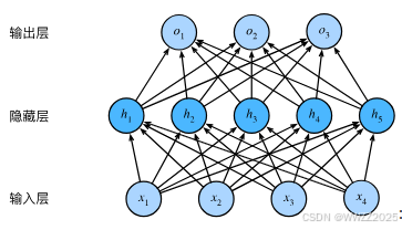
1.2 多层感知机(MLP, Multi-Layer Perceptron)
相较于感知机,多了隐藏层。需要激活函数激活,可以更近似的表示为目标非线性关系。激活函数详情如下2。
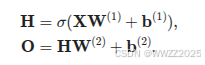
多层感知机经激活函数非线性化的公式为:
其中H为隐藏层非线性化后的输出,O为最终经非线性化后的输出。角标对应第几层。
PS.多层感知机与激活函数之间的关系
多层感知机输出是线性,经过激活函数将每一层输出非线性化后变为更加近似的目标函数
2 常见激活函数
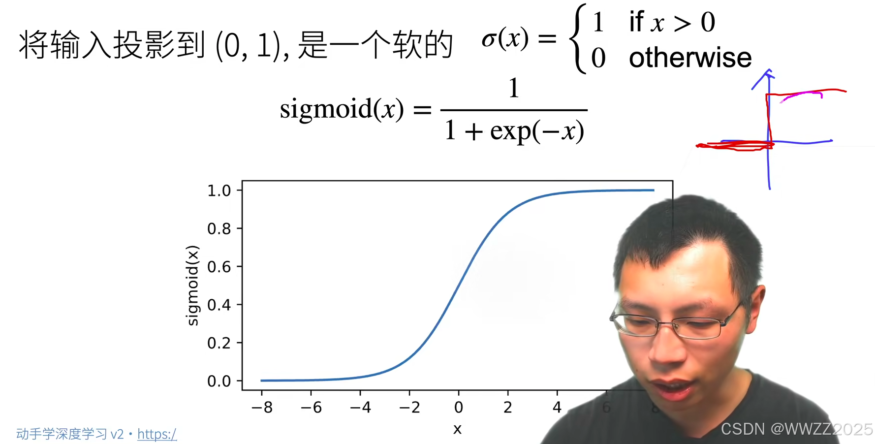
2.1 Sigmoid激活函数
2.2 Tanh激活函数

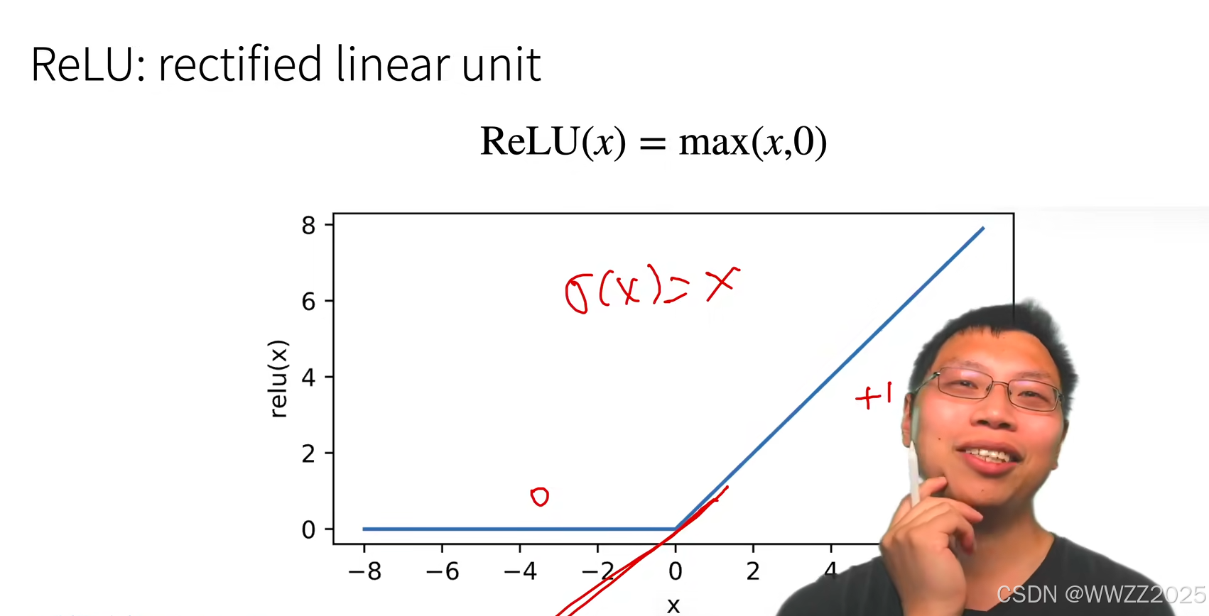
2.3 ReLU激活函数
3 多层感知机从零实现
3.1 导入库及数据集
import torch
from torch import nn
from d2l import torch as d2l
import torch.optim as optim
import matplotlib.pyplot as plt


batch_size = 256
train_iter, test_iter = d2l.load_data_fashion_mnist(batch_size)
3.2 初始化模型参数
# 定义多层感知机模型(MLP)
class MLP(nn.Module):
    def __init__(self, num_inputs, num_hiddens, num_outputs):
        super(MLP, self).__init__()
        self.flatten = nn.Flatten()  # 将输入展平成一维
        self.dense1 = nn.Linear(num_inputs, num_hiddens)  # 第一个全连接层
        self.relu = nn.ReLU()  # ReLU 激活函数
        self.dense2 = nn.Linear(num_hiddens, num_outputs)  # 第二个全连接层

    def forward(self, X):
        X = self.flatten(X)  # 展平输入
        X = self.relu(self.dense1(X))  # 第一个全连接层加 ReLU 激活
        return self.dense2(X)  # 第二个全连接层,输出
设置隐藏层和输出层的初始参数。
3.3 模型
# 创建模型
num_inputs, num_hiddens, num_outputs = 784, 256, 10
net = MLP(num_inputs, num_hiddens, num_outputs)
3.4 损失函数
loss = nn.CrossEntropyLoss(reduction='none')此处使用交叉熵损失函数,详见5.4.4:https://blog.csdn.net/weixin_45728280/article/details/153778299?spm=1001.2014.3001.5501
reduction参数,控制损失的汇总方式,分别为:'none','mean','sum'。其中'none'指返回每个样本的单独损失,'mean'指返回所有样本的平均损失,'sum'指返回所有样本损失的总和。
3.5 训练
# 准确度计算
def accuracy(y_hat, y):
    return (y_hat.argmax(dim=1) == y).float().sum().item()

# 评估准确率的函数
def evaluate_accuracy(net, data_iter):
    net.eval()  # 切换到评估模式
    metric = d2l.Accumulator(2)  # 存储正确预测和总数
    with torch.no_grad():  # 关闭梯度计算
        for X, y in data_iter:
            metric.add(accuracy(net(X), y), y.size(0))
    return metric[0] / metric[1]

# 自定义训练函数
def train_ch3(net, train_iter, test_iter, loss, num_epochs, updater):
    net.train()  # 切换到训练模式

    # 用于保存每轮的loss和accuracy
    train_losses = []
    train_accuracies = []
    test_accuracies = []

    for epoch in range(num_epochs):
        print(f"Epoch {epoch + 1}/{num_epochs}")
        train_acc, train_loss = 0.0, 0.0
        num_train_samples = 0

        for X, y in train_iter:
            y_hat = net(X)  # 前向传播
            l = loss(y_hat, y)  # 计算损失

            # 将损失转换为标量
            l = l.mean()  # 或者 l.sum() 根据需要选择

            updater.zero_grad()  # 清除梯度
            l.backward()  # 反向传播计算梯度
            updater.step()  # 更新参数

            # 累积准确度和损失
            train_acc += accuracy(y_hat, y)
            train_loss += l.item() * y.size(0)
            num_train_samples += y.size(0)

        # 打印每轮训练结果
        print(f"  Train Loss: {train_loss / num_train_samples:.4f}, Train Accuracy: {train_acc / num_train_samples:.4f}")

        # 评估每个epoch结束后模型在测试集上的表现
        test_acc = evaluate_accuracy(net, test_iter)
        print(f"  Test Accuracy: {test_acc:.4f}")

        # 记录每轮的结果
        train_losses.append(train_loss / num_train_samples)
        train_accuracies.append(train_acc / num_train_samples)
        test_accuracies.append(test_acc)

    # 返回训练过程中记录的结果
    return train_losses, train_accuracies, test_accuracies

# 优化器
lr = 0.1
updater = optim.SGD(net.parameters(), lr=lr)  # 使用nn.Module的parameters()获取模型参数

# 训练
num_epochs = 10
train_losses, train_accuracies, test_accuracies = train_ch3(net, train_iter, test_iter, loss, num_epochs, updater)
3.6 绘制图像
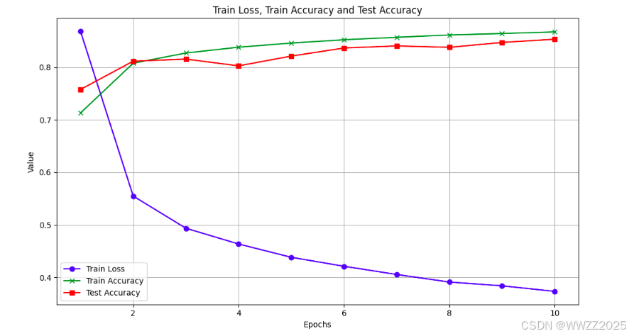
# 绘制训练损失、训练准确度和测试准确度的曲线
plt.figure(figsize=(10, 6))

# 绘制训练损失曲线
plt.plot(range(1, num_epochs + 1), train_losses, label='Train Loss', color='blue', linestyle='-', marker='o')

# 绘制训练准确度曲线
plt.plot(range(1, num_epochs + 1), train_accuracies, label='Train Accuracy', color='green', linestyle='-', marker='x')

# 绘制测试准确度曲线
plt.plot(range(1, num_epochs + 1), test_accuracies, label='Test Accuracy', color='red', linestyle='-', marker='s')

# 设置图表的标签和标题
plt.xlabel('Epochs')
plt.ylabel('Value')
plt.title('Train Loss, Train Accuracy and Test Accuracy')
plt.legend()  # 显示图例
plt.grid(True)  # 显示网格

# 显示图形
plt.tight_layout()
plt.show()
3.7 结果
Epoch 1/10
  Train Loss: 0.8688, Train Accuracy: 0.7132
  Test Accuracy: 0.7580
Epoch 2/10
  Train Loss: 0.5549, Train Accuracy: 0.8081
  Test Accuracy: 0.8119
Epoch 3/10
  Train Loss: 0.4935, Train Accuracy: 0.8275
  Test Accuracy: 0.8159
Epoch 4/10
  Train Loss: 0.4635, Train Accuracy: 0.8386
  Test Accuracy: 0.8030
Epoch 5/10
  Train Loss: 0.4382, Train Accuracy: 0.8465
  Test Accuracy: 0.8216
Epoch 6/10
  Train Loss: 0.4211, Train Accuracy: 0.8528
  Test Accuracy: 0.8370
Epoch 7/10
  Train Loss: 0.4054, Train Accuracy: 0.8574
  Test Accuracy: 0.8410
Epoch 8/10
  Train Loss: 0.3910, Train Accuracy: 0.8619
  Test Accuracy: 0.8383
Epoch 9/10
  Train Loss: 0.3838, Train Accuracy: 0.8646
  Test Accuracy: 0.8476
Epoch 10/10
  Train Loss: 0.3733, Train Accuracy: 0.8677
  Test Accuracy: 0.8538
4 多层感知机简洁实现
# 调用库
import torch
from torch import nn
from d2l import torch as d2l

#模型
net = nn.Sequential(nn.Flatten(),
                    nn.Linear(784, 256),
                    nn.ReLU(),
                    nn.Linear(256, 10))

def init_weights(m):
    if type(m) == nn.Linear:
        nn.init.normal_(m.weight, std=0.01)

net.apply(init_weights);

#导入数据集
batch_size, lr, num_epochs = 256, 0.1, 10
loss = nn.CrossEntropyLoss(reduction='none')
trainer = torch.optim.SGD(net.parameters(), lr=lr)

#定义训练函数
# 自定义 train_ch3 函数(完全兼容 d2l 的写法)
def train_ch3(net, train_iter, test_iter, loss, num_epochs, updater):
    # 定义一个精度计算函数
    def accuracy(y_hat, y):
        return (y_hat.argmax(dim=1) == y).float().mean().item()

    # 训练
    for epoch in range(num_epochs):
        # 训练模式
        net.train()
        total_loss, total_acc, total_num = 0.0, 0.0, 0

        for X, y in train_iter:
            y_hat = net(X)
            l = loss(y_hat, y).mean()
            updater.zero_grad()
            l.backward()
            updater.step()

            total_loss += l.item() * y.size(0)
            total_acc += (y_hat.argmax(1) == y).float().sum().item()
            total_num += y.size(0)

        train_loss = total_loss / total_num
        train_acc = total_acc / total_num
        test_acc = evaluate_accuracy(net, test_iter)

        print(f'epoch {epoch + 1}, loss {train_loss:.3f}, train acc {train_acc:.3f}, test acc {test_acc:.3f}')


# 定义测试精度评估函数
def evaluate_accuracy(net, data_iter):
    net.eval()
    acc_sum, n = 0.0, 0
    with torch.no_grad():
        for X, y in data_iter:
            acc_sum += (net(X).argmax(dim=1) == y).float().sum().item()
            n += y.size(0)
    return acc_sum / n

#训练
train_iter, test_iter = d2l.load_data_fashion_mnist(batch_size)
train_ch3(net, train_iter, test_iter, loss, num_epochs, trainer)
结果:

5 兼容性修正
5.1 安装
考虑版本兼容问题,安装兼容新版依赖的d2l版本:
pip install -U d2l==1.0.3
5.2 验证版本
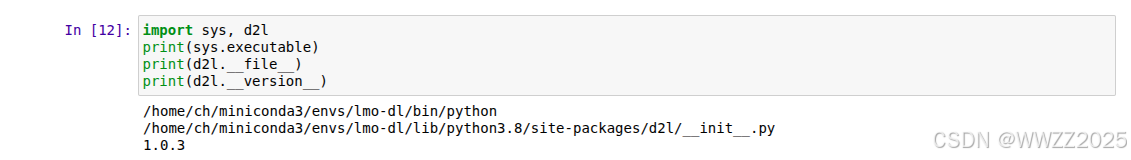
在jupyter notebook中新建一个单元格,输入下面代码,查看输出。注意在D2L V1.0.3以后,
train_ch3被移除,改成了更通用的train_ch13()
import sys, d2l
print(sys.executable)
print(d2l.__file__)
print(d2l.__version__)
5.3 测试代码
from d2l import torch as d2l
import torch
from torch import nn

# 1. 定义模型
net = nn.Sequential(
    nn.Flatten(),
    nn.Linear(784, 256),
    nn.ReLU(),
    nn.Linear(256, 10)
)

def init_weights(m):
    if type(m) == nn.Linear:
        nn.init.normal_(m.weight, std=0.01)
net.apply(init_weights)

# 2. 数据
batch_size, lr, num_epochs = 256, 0.1, 10
train_iter, test_iter = d2l.load_data_fashion_mnist(batch_size)

# 3. 损失函数和优化器
loss = nn.CrossEntropyLoss(reduction='none')
trainer = torch.optim.SGD(net.parameters(), lr=lr)

# 4. 显式传入 devices 参数
d2l.train_ch13(net, train_iter, test_iter, loss, trainer, num_epochs, devices=[d2l.try_gpu()])
