【视觉SLAM十四讲】后端 2

文章目录

- 滑动窗口
- - [边缘化与 Schur 补](#边缘化与 Schur 补)
  - [稀疏性的破坏（Fill in）](#稀疏性的破坏（Fill in）)
- 位姿图
- - 位姿图优化
  - [g2o 与位姿图优化](#g2o 与位姿图优化)
  - - [原生 g2o 代码实例](#原生 g2o 代码实例)
    - 李代数代码实例

后端 1 中提到如何构建 BA 问题，即同时优化所有的相机位姿和路径点，而本讲主要探讨的就是如何保证在大规模场景下 BA 的实时性

BA 的理想情况是将所有时刻的所有相机和路径点都放进 H H H 矩阵优化，但是随着时间的推移将产生大量数据，这将严重影响实时性乃至超出计算机的处理能力

为了解决此问题，有两种较为常见的方法

滑动窗口法：将 BA 固定在一个时间窗口，每当新的关键帧加入时，将窗口内最早的关键帧丢弃
共视图：仅优化与当前帧有足够共视路标点的关键帧

滑动窗口

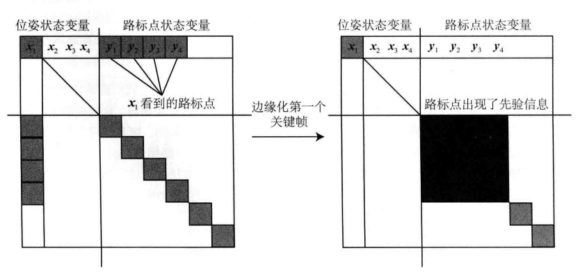
在使用滑动窗口算法的时候，当加入新的关键帧时，旧的关键帧的处理便成了问题，如果直接删除，那么这一帧的约束信息将直接消失，导致协方差估计过于乐观，降低精度。因此我们需要利用边缘化提炼出旧帧的信息保留下来

边缘化与 Schur 补

边缘化的本质是利用 Schur 补将被删除变量的信息投影到剩余变量上

回顾 BA 中的线性方程： H Δ x = g H\Delta x=g HΔx=g

H m m H m r H r m H r r \] ⋅ \[ Δ x m Δ x r \] = \[ b m b r \] \\begin{bmatrix} H_{mm}\&H_{mr}\\\\H_{rm}\&H_{rr} \\end{bmatrix} \\cdot \\begin{bmatrix} \\Delta x_{m}\\\\ \\Delta x_{r} \\end{bmatrix}= \\begin{bmatrix} b_{m}\\\\b_{r} \\end{bmatrix} \[HmmHrmHmrHrr\]⋅\[ΔxmΔxr\]=\[bmbr

x m x_{m} xm ：将被边缘化的变量
x r x_{r} xr ：保留的剩余变量
利用高斯消元得到关于 Δ x \Delta x Δx 的方程：
( H r r − H r m H m m − 1 H m r ) ⏟ H n e w Δ x r = b r − H r m H m m − 1 b m \underbrace{(H_{rr}-H_{rm}H_{mm}^{-1}H_{mr})}{H{new}}\Delta x_{r}=b_{r}-H_{rm}H^{-1}{mm}b{m} Hnew (Hrr−HrmHmm−1Hmr)Δxr=br−HrmHmm−1bm
H n e w H_{new} Hnew 即边缘化后剩余变量 x r x_{r} xr 的新信息矩阵
传递对象：
滑动窗口内较新的关键帧：如果新帧与被边缘化的旧帧观测到了相同的路标点，或者有直接的里程计约束，那么旧帧的信息会作为先验信息传递给新帧
滑动窗口内的路标点：更新被边缘化的旧帧观测的路标点位置

特性	BA	边缘化
场景	求解 H Δ x = g H\Delta x=g HΔx=g	移除旧帧并保留信息
消除变量	路标点 Δ x p \Delta x_{p} Δxp	旧关键帧 Δ x m \Delta x_{m} Δxm
保留变量	相机位姿 Δ x e \Delta x_{e} Δxe	剩余帧+路标 Δ x r \Delta x_{r} Δxr
Schur补	S = B − E C − 1 E T S=B-EC^{-1}E^T S=B−EC−1ET	H n e w = H r r − H r m H m m − 1 H m r H_{new}=H_{rr}-H_{rm}H^{-1}{mm}H{mr} Hnew=Hrr−HrmHmm−1Hmr
目的	加速计算，求解相机位姿	信息传递，将旧帧的约束传给新帧

S S S 矩阵其实就是边缘化掉路标点的相机位姿信息矩阵（ H n e w H_{new} Hnew）

稀疏性的破坏（Fill in）

让我们回忆一下后端 1 中提到的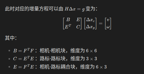

H = [ B E E T C ] H=\begin{bmatrix} B & E \\ E^T & C \end{bmatrix} \\ H=[BETEC]

其中 C 矩阵是对角块矩阵，因为路径点与路径点之间并无联系，所以仅有对角上用 3 × 3 3\times 3 3×3 矩阵存储路径点的信息矩阵，其余点都为0

对于对角矩阵 C i i C_{ii} Cii ，其存储的是所有相机关于该路标点位置的二阶导数之和 ，物理意义上，它描述的是该路标点的确定程度

路标点之间的无关性正是 C 矩阵稀疏性的来源，基于这点，BA 才能利用 Schur 消元加速计算

当我们使用边缘化移除旧帧 T o l d T_{old} Told 时：

T o l d T_{old} Told 同时观测到的所有路径点，都与 T o l d T_{old} Told 存在着约束
当我们边缘化 T o l d T_{old} Told 时，Schur 补会将这些点都联系起来
这意味着原先互不相关的路径点之间，产生了直接的数学联系
这将使得 C 矩阵中原先非对角的元素不再为 0 ，C 矩阵变成了稠密矩阵，在下一次 BA 过程中，无法利用 C 矩阵的稀疏性加速计算

位姿图

如果不希望处理复杂的边缘化，或者需要进行大范围的全局调整，可以采用位姿图优化。

位姿图优化的核心思想就是不再优化 BA 中的路标点，而是仅把它们看成对姿态节点的约束

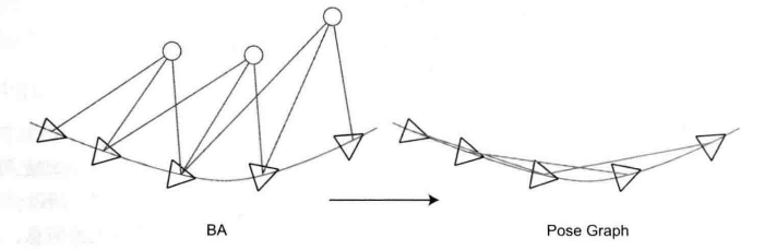
位姿图优化

位姿图中的节点标示相机位姿，以 T 1 , ⋯ , T n T_{1},\cdots,T_{n} T1,⋯,Tn 表示，边则是两个位姿节点之间的相对运动估计。

假设我们估计 T i T_{i} Ti 和 T j T_{j} Tj 之间的一个相对运动 T i j T_{ij} Tij ，表达式如下
T i j = T i − 1 T j T_{ij}=T_{i}^{-1}T_{j} Tij=Ti−1Tj

或者写成李代数形式（ ∘ \circ ∘ 表示"在李群上做逆和乘法，对应到李代数上的运算"， ∨ ^\vee ∨ 表示矩阵转向量）
Δ ξ i j = ξ i − 1 ∘ ξ j = ln ⁡ ( T i − 1 T j ) ∨ \Delta \xi_{ij}=\xi_{i}^{-1}\circ\xi_{j}=\ln(T_{i}^{-1}T_{j})^\vee Δξij=ξi−1∘ξj=ln(Ti−1Tj)∨

该等式不会严格成立，所以我们还要引入最小二乘，先构建误差项 e i j e_{ij} eij
e i j = ln ⁡ ( T i j − 1 T i − 1 T j ) ∨ e_{ij}=\ln(T^{-1}{ij}T^{-1}{i}T_{j})^\vee eij=ln(Tij−1Ti−1Tj)∨

T i j − 1 T_{ij}^{-1} Tij−1 ：两个相机之间的相对运动测量值
T i , T j T_{i},T_{j} Ti,Tj ：两个相机在世界坐标系下的估计位姿

理想情况下， T i j = T i − 1 T j T_{ij}=T_{i}^{-1}T_{j} Tij=Ti−1Tj
李群和李代数中提到过，李群无法直接做减法，这里用"乘逆"来表示减法

如果估计没有偏差， T i j − 1 ⋅ ( T i − 1 T j ) = I T_{ij}^{-1}\cdot(T_{i}^{-1}T_{j})=I Tij−1⋅(Ti−1Tj)=I

反之则是得到一个残差矩阵

要优化的变量有两个： ξ i \xi_{i} ξi 和 ξ j \xi_{j} ξj ，因此我们要求 e i j e_{ij} eij 关于这两个变量的导数，给 T i T_{i} Ti 和 T j T_{j} Tj 各自左乘扰动 δ ξ i \delta\xi_i δξi 和 δ ξ j \delta\xi_j δξj ，此时误差变为 ( ( A B ) − 1 = B − 1 A − 1 (AB)^{-1}=B^{-1}A^{-1} (AB)−1=B−1A−1)
e ^ i j = ln ⁡ ( T i j − 1 T i − 1 exp ⁡ ( − δ ξ i ∧ ) exp ⁡ ( δ ξ j ∧ ) ) ∨ \hat{e}{ij}=\ln\left(T{ij}^{-1}T_{i}^{-1}\exp\left(-\delta\xi_{i}^\wedge\right)\exp(\delta\xi_{j}^\wedge)\right)^\vee e^ij=ln(Tij−1Ti−1exp(−δξi∧)exp(δξj∧))∨

为了利用李群和李代数，我们需要将式子化为诸如 ln ⁡ ( A ⋅ exp ⁡ ( δ ∧ ) ) ∨ \ln(A\cdot \exp(\delta^\wedge))^\vee ln(A⋅exp(δ∧))∨ 的形式

定义 Δ ξ = d e f δ ξ j − δ ξ i \Delta\xi \stackrel{def}{=}\delta\xi_{j}-\delta\xi_{i} Δξ=defδξj−δξi

先进行线性近似 ( exp ⁡ ( A ) exp ⁡ ( B ) = exp ⁡ ( A + B ) ) (\exp(A)\exp(B)=\exp(A+B)) (exp(A)exp(B)=exp(A+B))，得到
e ^ i j ≈ ln ⁡ ( T i j − 1 T i − 1 exp ⁡ ( Δ ξ ∧ ) T j ) ∨ \hat{e}{{ij}}\approx\ln\left(T{ij}^{-1}T_{i}^{-1}\exp\left(\Delta\xi^\wedge\right)T_{j}\right)^\vee e^ij≈ln(Tij−1Ti−1exp(Δξ∧)Tj)∨

在下一步推导之前，我们还需要了解一下**共轭和伴随性质**

不过 T i − 1 exp ⁡ ( ( Δ ξ ) ∧ ) T j T_{i}^{-1}\exp\left((\Delta\xi)^\wedge\right)T_{j} Ti−1exp((Δξ)∧)Tj 并不是一个共轭式子，只是一个约束链，因为共轭式子的要求是左右两侧的矩阵必须是互为逆的同一位姿，但这里是不同时刻的两个位姿

先来剖析一下这个式子：
P j ⏟ j 坐标系 → T j P W ⏟ 世界坐标系 → exp ⁡ ( Δ ξ ∧ ) P W ′ ⏟ 施加扰动后 → T i − 1 P i ⏟ i 坐标系 \underbrace{ P_{j} }{ j~\text{}{坐标系} } \xrightarrow{T{j}} \underbrace{ P_{W} }{ \text{世界坐标系} } \xrightarrow{\exp(\Delta\xi^\wedge)}\underbrace{ P{W}' }{ \text{施加扰动后} } \xrightarrow{T{i}^{-1}} \underbrace{ P_{i} }_{ i~\text{坐标系} } j 坐标系 PjTj 世界坐标系 PWexp(Δξ∧) 施加扰动后 PW′Ti−1 i 坐标系 Pi

这显然不满足条件，因为误差项应当是在 j 坐标系下的，所以还要利用伴随性质纠正坐标系转换

已知：
exp ⁡ ( ξ ∧ ) T = T exp ⁡ ( ( A d ( T − 1 ) ξ ) ∧ ) \exp(\xi^\wedge)T=T\exp\left((Ad(T^{-1})\xi)^\wedge\right) exp(ξ∧)T=Texp((Ad(T−1)ξ)∧)

此时可以凑出标准的 BCH 形式
e ^ i j = ln ⁡ ( T i j − 1 T i − 1 T j ⏟ E i j （原误差） ⋅ exp ⁡ ( ( A d ( T j − 1 ) Δ ξ ) ∧ ⏟ 转换后扰动 ) ) ∨ \hat{e}{ij}=\ln\left(\underbrace{ T{ij}^{-1}T_{i}^{-1}T_{j} }{ E{ij} \text{（原误差）}}\cdot \exp\left(\underbrace{ (Ad(T_{j}^{-1})\Delta \xi)^\wedge}_{ \text{转换后扰动} }\right)\right)^\vee e^ij=ln Eij（原误差） Tij−1Ti−1Tj⋅exp 转换后扰动 (Ad(Tj−1)Δξ)∧ ∨

根据 S E ( 3 ) SE(3) SE(3) 上的 BCH 近似：
ln ⁡ ( A ⋅ exp ⁡ ( δ ∧ ) ) ∨ ≈ ln ⁡ ( A ) ∨ + J r − 1 ( ln ⁡ ( A ) ∨ ) ⋅ δ \ln(A\cdot \exp(\delta^\wedge))^\vee \approx \ln(A)^\vee+J_{r}^{-1}(\ln(A)^\vee)\cdot\delta ln(A⋅exp(δ∧))∨≈ln(A)∨+Jr−1(ln(A)∨)⋅δ

代入得到最终的线性化误差公式：
e ^ i j ≈ e i j + J r − 1 ( e i j ) ⋅ A d ( T j − 1 ⋅ Δ ξ ) \hat{e}{ij}\approx e{ij}+J_{r}^{-1}(e_{ij})\cdot Ad(T_{j}^{-1}\cdot\Delta \xi) e^ij≈eij+Jr−1(eij)⋅Ad(Tj−1⋅Δξ)

展开得到
e ^ i j ≈ e i j + J r − 1 ( e i j ) A d ( T j − 1 ) ⋅ δ ξ j ⏟ 对 j 的导数项 − J r − 1 ( e i j ) A d ( T j − 1 ) ⋅ δ ξ i ⏟ 对 i 的导数项 \hat{e}{ij}\approx e{ij}+\underbrace{ J_{r}^{-1}(e_{ij})Ad(T^{-1}{j})\cdot\delta \xi{j} }{ \text{对} j \text{的导数项} }-\underbrace{ J{r}^{-1}(e_{ij})Ad(T_{j}^{-1})\cdot\delta \xi_{i} }_{ \text{对 } i \text{ 的导数项} } e^ij≈eij+对j的导数项 Jr−1(eij)Ad(Tj−1)⋅δξj−对 i 的导数项 Jr−1(eij)Ad(Tj−1)⋅δξi

于是我们得到了误差关于两个位姿的雅可比矩阵

对 T i T_{i} Ti 的雅可比：
∂ e i j ∂ δ ξ i = − J r − 1 ( e i j ) ⋅ A d ( T j − 1 ) \frac{\partial e_{ij}}{\partial\delta \xi_{i}}=-J_{r}^{-1}(e_{ij})\cdot Ad(T_{j}^{-1}) ∂δξi∂eij=−Jr−1(eij)⋅Ad(Tj−1)
对 T j T_{j} Tj 的雅可比： ∂ e i j ∂ δ ξ j = J r − 1 ( e i j ) ⋅ A d ( T j − 1 ) \frac{\partial e_{ij}}{\partial\delta \xi_{j}}=J_{r}^{-1}(e_{ij})\cdot Ad(T_{j}^{-1}) ∂δξj∂eij=Jr−1(eij)⋅Ad(Tj−1)
由于 s e ( 3 ) \mathfrak{se}(3) se(3) 上的左右雅可比形式过于复杂，所以通常会取近似值，当误差接近于 0 时，我们可以近似其为 I I I 或
J r − 1 ( e i j ) ≈ I + 1 2 [ ϕ e ∧ ρ e ∧ 0 ϕ e ∧ ] J_{r}^{-1}(e_{ij}) \approx I + \frac{1}{2}\begin{bmatrix}\phi_{e}^\wedge&\rho_{e}^\wedge\\0&\phi_{e}^\wedge\end{bmatrix} Jr−1(eij)≈I+21[ϕe∧0ρe∧ϕe∧]
不用过于担心近似引进的误差，因为在迭代算法里，我们其实需求的不是实际精确的值，而是一个优化方向，而且随着迭代的推进，误差减小的时候，雅可比矩阵也会靠近我们近似的 I I I

g2o 与位姿图优化

\[g2o入门\]

原生 g2o 代码实例

cpp 复制代码

#include <iostream>
#include <memory>
#include <eigen3/Eigen/Core>
#include <eigen3/Eigen/Geometry>
#include <sophus/se3.hpp>
#include <sophus/so3.hpp>
#include <g2o/core/base_binary_edge.h>
#include <g2o/core/base_vertex.h>
#include <g2o/core/block_solver.h>
#include <g2o/core/optimization_algorithm_levenberg.h>
#include <g2o/solvers/dense/linear_solver_dense.h>
#include <g2o/types/slam3d/vertex_se3.h>
#include <g2o/types/slam3d/edge_se3.h>

int main()
{
    // 1. 数据生成
    // 半径 10 米的圆周轨迹，每步走一度
    std::vector<Eigen::Isometry3d> poses;
    double radius = 10.0;
    for (int i = 0; i < 360; i++)
    {
        double theta = i * M_PI / 180.0;
        // 位置
        Eigen::Vector3d trans(radius * cos(theta), radius * sin(theta), 0);
        // 姿态
        Eigen::Quaterniond q;
        q = Eigen::AngleAxisd(theta + M_PI_2, Eigen::Vector3d::UnitZ());

        Eigen::Isometry3d pose = Eigen::Isometry3d::Identity();
        pose.rotate(q);
        pose.pretranslate(trans);
        poses.push_back(pose);
    }

    // 2. 构建 g2o 优化器
    typedef g2o::BlockSolver<g2o::BlockSolverTraits<6, 6>> BlockSolverType;

    typedef g2o::LinearSolverDense<BlockSolverType::PoseMatrixType> LinearSolverType;

    auto solver = std::make_unique<g2o::OptimizationAlgorithmLevenberg>(
        std::make_unique<BlockSolverType>(std::make_unique<LinearSolverType>())
    );

    g2o::SparseOptimizer optimizer;
    optimizer.setAlgorithm(solver.release());
    optimizer.setVerbose(true);

    // 3. 添加位姿顶点
    // 添加噪声
    Eigen::Isometry3d current_pose = poses[0];

    // 随机数生成器
    double trans_noise = 0.1;  // 平移噪声标准差
    double rot_noise = 0.01;   // 旋转噪声标准

    for (int i = 0; i < poses.size(); i++)
    {
        g2o::VertexSE3* v = new g2o::VertexSE3();
        v->setId(i);

        if (i == 0)
        {
            v->setEstimate(current_pose);
            v->setFixed(true); // 固定第一个位姿
        }
        else
        {
            // 计算相对运动真实值
            Eigen::Isometry3d relative_motion = poses[i - 1].inverse() * poses[i];

            // 添加噪声
            Eigen::Vector3d noise_trans = Eigen::Vector3d::Random() * trans_noise;
            Eigen::Vector3d noise_rot = Eigen::Vector3d::Random() * rot_noise;
            Eigen::Quaterniond noise_q = Sophus::SO3d::exp(noise_rot).unit_quaternion();

            Eigen::Isometry3d noisy_relative_motion = Eigen::Isometry3d::Identity();
            noisy_relative_motion.rotate(noise_q * relative_motion.rotation());
            noisy_relative_motion.pretranslate(relative_motion.translation() + noise_trans);

            // 更新当前位姿
            current_pose = current_pose * noisy_relative_motion;
            v->setEstimate(current_pose);

            // 添加边
            auto edge = std::make_unique<g2o::EdgeSE3>();
            edge->setVertex(0, optimizer.vertex(i - 1));
            edge->setVertex(1, v);
            edge->setMeasurement(noisy_relative_motion);

            // 信息矩阵
            Eigen::Matrix<double, 6, 6> information = Eigen::Matrix<double, 6, 6>::Identity();
            information.block<3,3>(0, 0) *= 1.0 / (trans_noise * trans_noise);
            information.block<3,3>(3, 3) *= 1.0 / (rot_noise * rot_noise);
            edge->setInformation(information);

            optimizer.addEdge(edge.release());
        }
        optimizer.addVertex(v);
    }

    auto* last_vertex = static_cast<g2o::VertexSE3*>(optimizer.vertex(359));
    Eigen::Vector3d end_error = last_vertex->estimate().translation() - poses[359].translation();
    std::cout << "Before optimization: End pose error distance = " 
              << end_error.norm() 
              << " m" << std::endl;

    // 添加回环边
    g2o::EdgeSE3* loop_edge = new g2o::EdgeSE3();
    loop_edge->setVertex(0, optimizer.vertex(359)); // 回环到第一个顶点
    loop_edge->setVertex(1, optimizer.vertex(0));

    Eigen::Isometry3d loop_measurement = poses[359].inverse() * poses[0];
    loop_edge->setMeasurement(loop_measurement);

    Eigen::Matrix<double, 6, 6> loop_information = Eigen::Matrix<double, 6, 6>::Identity() * 1000.0;
    loop_edge->setInformation(loop_information);

    optimizer.addEdge(loop_edge);

    // 4. 优化
    std::cout << "Start optimization" << std::endl;
    optimizer.initializeOptimization();
    optimizer.optimize(100);    

    auto* new_last_vertex = static_cast<g2o::VertexSE3*>(optimizer.vertex(359));
    Eigen::Vector3d new_end_error = new_last_vertex->estimate().translation() - poses[359].translation();
    std::cout << "After optimization: End pose error distance = " 
              << new_end_error.norm() 
              << " m" << std::endl;

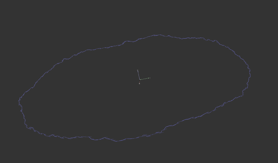
    optimizer.save("pose_graph_result.g2o");
}

效果图如下：

李代数代码实例

cpp 复制代码

#include <iostream>
#include <fstream>
#include <string>
#include <memory>
#include <eigen3/Eigen/Core>
#include <eigen3/Eigen/Geometry>
#include <sophus/se3.hpp>

#include <g2o/core/base_vertex.h>
#include <g2o/core/base_binary_edge.h>
#include <g2o/core/block_solver.h>
#include <g2o/core/optimization_algorithm_levenberg.h>
#include <g2o/solvers/eigen/linear_solver_eigen.h>

#include <g2o/core/factory.h>
#include <g2o/stuff/command_args.h>

typedef Eigen::Matrix<double, 6, 6> Matrix6d;
typedef Eigen::Matrix<double, 6, 1> Vector6d;

// J_R^{-1} 的近似
Matrix6d JRinv(const Sophus::SE3d& e)
{
    Matrix6d J;
    J.block(0, 0, 3, 3) = Sophus::SO3d::hat(e.so3().log());
    J.block(0, 3, 3, 3) = Sophus::SO3d::hat(e.translation());
    J.block(3, 0, 3, 3) = Eigen::Matrix3d::Zero();
    J.block(3, 3, 3, 3) = Sophus::SO3d::hat(e.so3().log());
    J = J * 0.5 + Matrix6d::Identity();
    return J;
}

class VertexSE3LieAlgebra : public g2o::BaseVertex<6, Sophus::SE3d>
{
public:
    EIGEN_MAKE_ALIGNED_OPERATOR_NEW

    virtual void setToOriginImpl() override
    {
        _estimate = Sophus::SE3d();
    }

    virtual void oplusImpl(const double* update) override
    {
        Vector6d update_eigen;
        update_eigen << update[0], update[1], update[2], update[3], update[4], update[5];
        _estimate = Sophus::SE3d::exp(update_eigen) * _estimate;
    }

    virtual bool read(std::istream& in) override
    {
        double data[7];
        for (int i = 0; i < 7; i++)
            in >> data[i];
        setEstimate(Sophus::SE3d(
            Eigen::Quaterniond(data[6], data[3], data[4], data[5]).normalized(),
            Eigen::Vector3d(data[0], data[1], data[2])
        ));
        return true;
    }

    virtual bool write(std::ostream& os) const override
    {
        Eigen::Quaterniond q = _estimate.unit_quaternion();
        os << _estimate.translation().transpose() << " ";
        os << q.x() << " " << q.y() << " " << q.z() << " " << q.w() << std::endl;
        return true;
    }
};

// 
class EdgeSE3LieAlgebra : public g2o::BaseBinaryEdge<6, Sophus::SE3d, VertexSE3LieAlgebra, VertexSE3LieAlgebra> {
public:
    EIGEN_MAKE_ALIGNED_OPERATOR_NEW

    virtual void computeError() override
    {
        Sophus::SE3d v1 = (static_cast<VertexSE3LieAlgebra*>(_vertices[0]))->estimate();
        Sophus::SE3d v2 = (static_cast<VertexSE3LieAlgebra*>(_vertices[1]))->estimate();
        
        _error = (_measurement.inverse() * (v1.inverse() * v2)).log();
    }

    // 雅可比计算（ J_r^{-1} \approx I）
    virtual void linearizeOplus() override
    {
        Sophus::SE3d v2 = (static_cast<VertexSE3LieAlgebra*>(_vertices[1]))->estimate();
        
        Matrix6d J = JRinv(Sophus::SE3d::exp(_error));
        J = J * v2.inverse().Adj();

        _jacobianOplusXi = -J;
        _jacobianOplusXj = J;
    }

    virtual bool read(std::istream& in) override
    {
        double data[7];
        for (int i = 0; i < 7; i++)
            in >> data[i];
        Eigen::Quaterniond q(data[6], data[3], data[4], data[5]);
        q.normalize();
        setMeasurement(Sophus::SE3d(
            q,
            Eigen::Vector3d(data[0], data[1], data[2])
        ));

        for (int i = 0; i < information().rows(); i++)
        {
            for (int j = 0; j < information().cols(); j++)
            {
                in >> information()(i, j);
                // 保持对称性
                if (i != j)
                {
                    information()(j, i) = information()(i, j);
                }
            }
        }

        return true;
    }

    virtual bool write(std::ostream& os) const override
    {
        VertexSE3LieAlgebra *v1 = static_cast<VertexSE3LieAlgebra*>(_vertices[0]);
        VertexSE3LieAlgebra *v2 = static_cast<VertexSE3LieAlgebra*>(_vertices[1]);

        Eigen::Quaterniond q = _measurement.unit_quaternion();
        os << _measurement.translation().transpose() << " ";
        os << q.x() << " " << q.y() << " " << q.z() << " " << q.w() << " ";
        for (int i = 0; i < information().rows(); ++i)
        {
            for (int j = i; j < information().cols(); ++j)
            {
                os << information()(i, j) << " ";
            }
        }
        os << std::endl;
        return true;
    }
};

int main()
{
    // 1. 读取位姿图
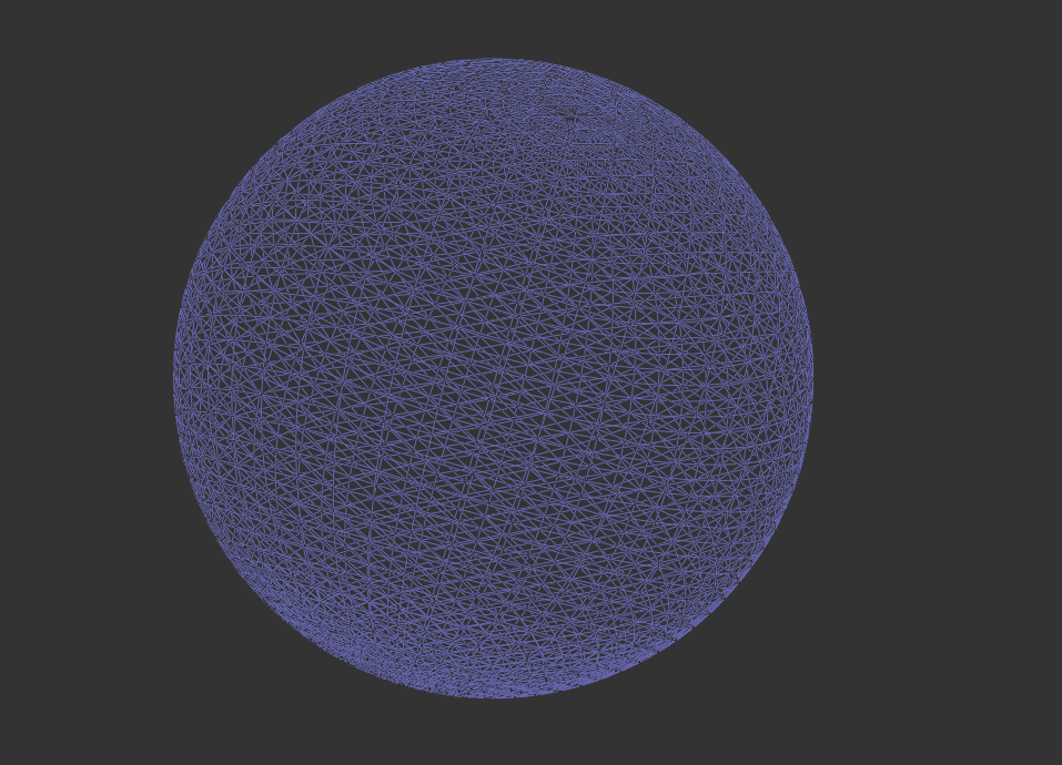
    std::fstream fin("../example/sphere.g2o");
    if (!fin)
    {
        std::cerr << "File not found." << std::endl;
        return -1;
    }

    // 2. 构建优化器
    typedef g2o::BlockSolver<g2o::BlockSolverTraits<6, 6>> BlockSolverType;
    typedef g2o::LinearSolverEigen<BlockSolverType::PoseMatrixType> LinearSolverType;

    auto solver = new g2o::OptimizationAlgorithmLevenberg(
        std::make_unique<BlockSolverType>(std::make_unique<LinearSolverType>())
    );

    g2o::SparseOptimizer optimizer;
    optimizer.setAlgorithm(solver);
    optimizer.setVerbose(true);

    // 3. 从文件中加载顶点和边
    int vertex_count = 0, edge_count = 0;
    while (!fin.eof())
    {
        std::string name;
        fin >> name;
        if (name == "VERTEX_SE3:QUAT")
        {
            int idx = 0;
            double data[7];
            fin >> idx;
            for (int i = 0; i < 7; i++)
                fin >> data[i];

            Eigen::Quaterniond q(data[6], data[3], data[4], data[5]);
            q.normalize();
            Eigen::Vector3d t(data[0], data[1], data[2]);   
            Sophus::SE3d pose(q, t);

            VertexSE3LieAlgebra* v = new VertexSE3LieAlgebra();
            v->setId(idx);
            v->setEstimate(pose);
            optimizer.addVertex(v);
            vertex_count++;

            if (idx == 0)
                v->setFixed(true); // 固定第一个节点
        }
        else if (name == "EDGE_SE3:QUAT")
        {
            int idx1, idx2;
            fin >> idx1 >> idx2;
            double data[7];
            for (int i = 0; i < 7; ++i)
                fin >> data[i];

            Eigen::Quaterniond q(data[6], data[3], data[4], data[5]);
            q.normalize();
            Eigen::Vector3d t(data[0], data[1], data[2]);
            Sophus::SE3d measurement(q, t);

            Matrix6d information = Matrix6d::Zero();
            for (int i = 0; i < 6; i++)
            {
                for (int j = i; j < 6; j++)
                {
                    fin >> information(i, j);
                    if (i != j)
                        information(j, i) = information(i, j);
                }
            }

            EdgeSE3LieAlgebra* e = new EdgeSE3LieAlgebra();
            e->setVertex(0, optimizer.vertex(idx1));
            e->setVertex(1, optimizer.vertex(idx2));
            e->setMeasurement(measurement);
            e->setInformation(information);
            optimizer.addEdge(e);
            edge_count++;
        }

        if (!fin.good())
            break;
    }

    std::cout << "Read total " << vertex_count << " vertices, " << edge_count << " edges." << std::endl;

    // 4. 优化
    std::cout << "Start optimization" << std::endl;
    optimizer.initializeOptimization();
    optimizer.optimize(100);

    // 5. 保存结果
    optimizer.save("sphere_se3_result.g2o");
}

G2O_REGISTER_TYPE_NAME("VERTEX_SE3:QUAT", VertexSE3LieAlgebra);
G2O_REGISTER_TYPE_NAME("EDGE_SE3:QUAT", EdgeSE3LieAlgebra);

优化前

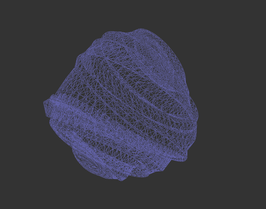
优化后