MSAC 算法详解以及与 RANSAC 对比示例

前文RANSAC算法------看完保证你理解中已经阐述了关于RANSAC算法的原理以及示例。

在许多含有噪声和异常点outliers 的数据拟合任务中，普通最小二乘法容易被异常点拉偏。RANSAC 可以在存在外点时稳健拟合，但在 near-outliers 情况下，它可能被误收内点，导致模型偏移。

MSAC（M-Estimator Sample Consensus） 是 RANSAC 的扩展，通过 残差代价 选择模型，而不仅仅依赖内点数量，从而获得更精确、稳定的拟合结果。

1. MSAC 算法详解

1.1 基本思想

MSAC 是 RANSAC 的自然扩展版本，核心目标是：

在含有外点的数据中，找到一组模型参数，使得整体残差代价最小，而不仅仅是最大化内点数量。

MSAC 的主要创新点在于 代价函数：

Cost = ∑ i = 1 N ρ ( e i ) \text{Cost} = \sum_{i=1}^{N} \rho(e_i) Cost=i=1∑Nρ(ei)

其中：

e i e_i ei 为第 i i i 个数据点到模型的残差；
ρ ( e i ) \rho(e_i) ρ(ei) 为 M-估计损失函数：

ρ ( e i ) = { e i 2 , if e i < threshold threshold 2 , if e i ≥ threshold \rho(e_i) = \begin{cases} e_i^2, & \text{if } e_i < \text{threshold} \\ \text{threshold}^2, & \text{if } e_i \geq \text{threshold} \end{cases} ρ(ei)={ei2,threshold2,if ei<thresholdif ei≥threshold

相比 RANSAC只计算内点数量，MSAC 将内点残差平方和阈值外点固定罚值都纳入考量，使得模型选择更加精细。

1.2 核心步骤

随机采样最小样本集
拟合模型
计算代价：内点残差平方，超出阈值点固定惩罚
更新最优模型：代价最小
重复迭代：直到达到最大迭代次数或置信度

可以理解为：RANSAC 关注"数量"，MSAC 关注"质量"。

1.3 MSAC 与 RANSAC 对比

特性	RANSAC	MSAC
模型评估	内点数量	残差代价（M-估计）
对 near-outliers 敏感	容易拉偏	稳健，可减小偏移
优势场景	外点比例高、模型简单	多模型竞争、复杂噪声场景
适用性	快速粗略估计	高精度鲁棒拟合

1.4 应用场景

MSAC 在计算机视觉和机器人领域非常实用：

相机标定：拟合内外参模型，剔除误匹配点
基础矩阵 / 单应性矩阵估计：点对中存在噪声和外点
点云拟合：3D 平面或曲面拟合，剔除异常点
自动驾驶：车道线或地面平面拟合，噪声点和遮挡点可控
SLAM / SfM：关键点匹配中剔除错误匹配

MSAC 适合任何需要鲁棒拟合、关注模型整体残差而不仅仅是内点数量的场景。

1.5 优劣势

优点：

在 near-outliers 情况下保持稳定
模型拟合更贴近真实分布
对残差大小敏感，可精细选择最优模型

缺点：

相比 RANSAC 计算稍复杂，需要累积残差代价
对阈值敏感，需要合理设置
当外点极端大时，MSAC 和 RANSAC 差异不明显

总结：MSAC 是 RANSAC 的"进化版"，更关注拟合质量，非常适合高精度与噪声复杂的任务。

2. 可视化示例

我们用一个简单的二维线性拟合实验展示 RANSAC 和 MSAC 的差异：

数据特点

主直线：y = 2.5x - 1.0
内点：添加小噪声
near-outliers：数量较多、略偏离真实直线，接近 RANSAC 阈值

3. Python3 完整示例（WSL 可保存图片）

python 复制代码

#!/usr/bin/env python3
# -*- coding: utf-8 -*-

import numpy as np
import random
import matplotlib
matplotlib.use("Agg")
import matplotlib.pyplot as plt

# 固定随机种子
np.random.seed(42)
random.seed(42)

# 数据生成
def generate_data():
    X = np.linspace(0, 10, 60)
    y_true = 2.5 * X - 1.0
    y_inliers = y_true + np.random.normal(0, 0.3, size=X.shape)
    X_near = np.linspace(0, 10, 40)
    y_near = 2.5 * X_near - 1.0 + np.random.normal(1.5, 0.5, size=X_near.shape)
    X_all = np.concatenate([X, X_near])
    y_all = np.concatenate([y_inliers, y_near])
    points = list(zip(X_all, y_all))
    return points, X_all, y_all, y_true

# 拟合直线
def fit_line(points):
    xs = np.array([p[0] for p in points])
    ys = np.array([p[1] for p in points])
    a, b = np.polyfit(xs, ys, 1)
    return a, b

# RANSAC
def ransac(points, iterations=200, threshold=2.0):
    best_model = None
    best_inliers = []
    for _ in range(iterations):
        sample = random.sample(points, 2)
        a, b = fit_line(sample)
        inliers = [(x, y) for x, y in points if abs(y - (a*x + b)) < threshold]
        if len(inliers) > len(best_inliers):
            best_inliers = inliers
            best_model = (a, b)
    return best_model, best_inliers

# MSAC
def msac(points, iterations=200, threshold=2.0):
    best_model = None
    best_cost = float("inf")
    for _ in range(iterations):
        sample = random.sample(points, 2)
        a, b = fit_line(sample)
        cost = sum((y - (a*x + b))**2 if abs(y-(a*x+b))<threshold else threshold**2
                   for x, y in points)
        if cost < best_cost:
            best_cost = cost
            best_model = (a, b)
    return best_model, best_cost

# MSE评估
def mse(model, points):
    a, b = model
    return np.mean([(y - (a*x + b))**2 for x, y in points])

# 主程序
if __name__ == "__main__":
    points, X_all, y_all, y_true = generate_data()

    ransac_model, ransac_inliers = ransac(points)
    msac_model, msac_cost = msac(points)

    print("=== Model parameters ===")
    print("True line:     y = 2.5x - 1.0")
    print(f"RANSAC line:   y = {ransac_model[0]:.3f}x + {ransac_model[1]:.3f}")
    print(f"MSAC line:     y = {msac_model[0]:.3f}x + {msac_model[1]:.3f}")
    print("\n=== Error comparison ===")
    print(f"RANSAC MSE: {mse(ransac_model, points):.4f}")
    print(f"MSAC MSE:   {mse(msac_model, points):.4f}")

    # 可视化保存
    plt.figure(figsize=(8,5))
    plt.scatter(X_all, y_all, s=10, color="gray", label="data")
    X_plot = np.linspace(0,10,100)
    plt.plot(X_plot, 2.5*X_plot-1, "k--", label="Ground truth")
    plt.plot(X_plot, ransac_model[0]*X_plot + ransac_model[1], "b", label="RANSAC")
    plt.plot(X_plot, msac_model[0]*X_plot + msac_model[1], "r", label="MSAC")
    plt.legend()
    plt.title("RANSAC vs MSAC (near-outliers visible)")
    plt.xlabel("x")
    plt.ylabel("y")
    plt.tight_layout()
    plt.savefig("ransac_vs_msac.png", dpi=150)
    plt.close()
    print("\nFigure saved to: ransac_vs_msac.png")

4. 运行效果

终端输出示例：

复制代码

=== Model parameters ===
True line:     y = 2.5x - 1.0
RANSAC line:   y = 2.549x + -1.312
MSAC line:     y = 2.504x + -1.072

=== Error comparison ===
RANSAC MSE: 0.6098
MSAC MSE:   0.5986

Figure saved to: ransac_vs_msac.png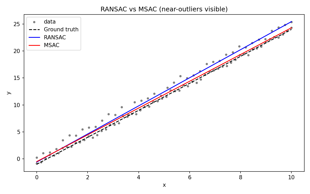

灰色散点：数据

黑色虚线：真实直线

蓝色：RANSAC（被 near-outliers 拉偏）

红色：MSAC（贴近真实线）

5. 总结

1. MSAC 优势：

在 near-outliers 或多模型竞争场景下稳健
不仅考虑内点数量，还关注残差平方

2. RANSAC 优势：

简单快速
对内点占比高的任务已足够

3.可视化实验：

near-outliers 会显著拉偏 RANSAC
MSAC 拟合更接近真实模型
MSAC 是 RANSAC 的自然升级，适用于自动驾驶、点云拟合、相机标定等高精度任务。