基于二维小波变换的图像增强MATLAB代码

%% 二维小波变换的图像增强（彩色图像）- 修复版
clear all; close all; clc;

%% 1. 读取彩色图像
img_original = imread('test1.jpeg'); % 使用内置彩色图像
if size(img_original, 3) ~= 3
    error('请使用彩色图像！');
end

figure('Name', '原始图像');
imshow(img_original); title('原始彩色图像');

%% 2. 将图像转换到适合处理的空间
% 方法1：YCbCr空间（推荐，保持色彩最自然）
img_ycbcr = rgb2ycbcr(img_original);
Y = im2double(img_ycbcr(:,:,1));  % 亮度分量
Cb = img_ycbcr(:,:,2);            % 色度分量
Cr = img_ycbcr(:,:,3);            % 色度分量

%% 3. 对亮度分量进行小波阈值增强
wavelet_name = 'sym4';
level = 2;

% 小波分解
[C, S] = wavedec2(Y, level, wavelet_name);

% 设置阈值参数
threshold_type = 's';  % 可选 's' (soft) 或 'h' (hard)
threshold_factor = 0.3;   % 阈值因子，可调整

% 计算全局阈值
T = threshold_factor * max(abs(C));

% 应用阈值
C_thresh = wthresh(C, threshold_type, T);

% 小波重构
Y_enhanced = waverec2(C_thresh, S, wavelet_name);

% 确保值在[0,1]范围内
Y_enhanced = min(max(Y_enhanced, 0), 1);

%% 4. 恢复色彩并转换回RGB
% 使用YCbCr空间
img_ycbcr_enhanced = img_ycbcr;
img_ycbcr_enhanced(:,:,1) = im2uint8(Y_enhanced); % 更新亮度分量

% 转换回RGB
img_enhanced = ycbcr2rgb(img_ycbcr_enhanced);

%% 5. 显示结果
figure('Name', '阈值增强后恢复原色', 'Position', [100, 100, 1200, 400]);

subplot(1, 3, 1);
imshow(img_original); 
title('原始彩色图像');
colorbar('southoutside');

subplot(1, 3, 2);
imshow(img_enhanced);
title(['阈值增强图像 (因子=', num2str(threshold_factor), ')']);
colorbar('southoutside');

subplot(1, 3, 3);
% 显示亮度分量增强对比
montage({Y, Y_enhanced}, 'Size', [1, 2]);
title('亮度分量增强对比 (左:原始, 右:增强)');
colorbar('southoutside');

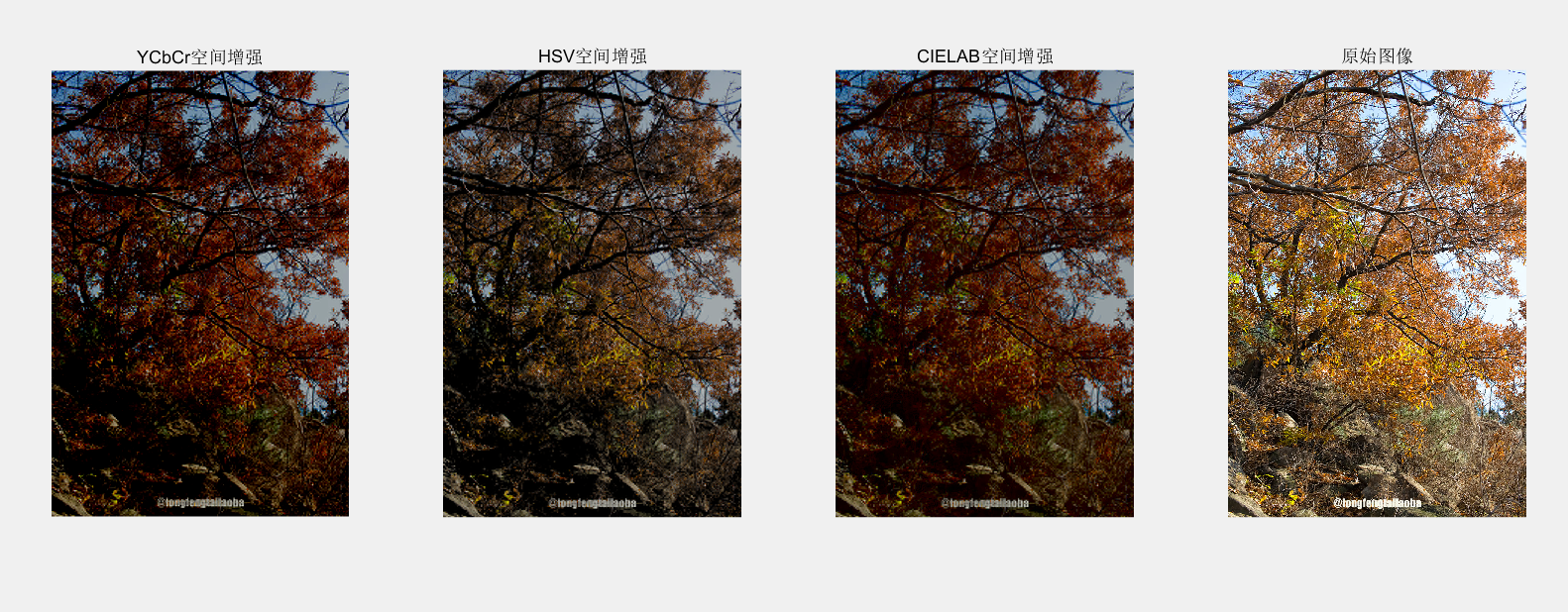
%% 6. 对比不同颜色空间的增强效果
methods = {'ycbcr', 'hsv', 'lab'};
titles = {'YCbCr空间增强', 'HSV空间增强', 'CIELAB空间增强'};

figure('Name', '不同颜色空间增强对比', 'Position', [100, 100, 1400, 400]);

for i = 1:length(methods)
    try
        img_method = wavelet_color_enhance(img_original, methods{i}, 'sym4', 2, 0.3);
        subplot(1, length(methods)+1, i);
        imshow(img_method);
        title(titles{i});
    catch
        subplot(1, length(methods)+1, i);
        imshow(img_original);
        title([methods{i}, '方法不可用']);
    end
end

% 显示原始图像
subplot(1, length(methods)+1, length(methods)+1);
imshow(img_original);
title('原始图像');

%% 7. 调用自适应增强
img_adaptive = adaptive_wavelet_enhance(img_original);

figure('Name', '自适应阈值增强');
subplot(1, 2, 1);
imshow(img_original);
title('原始图像');

subplot(1, 2, 2);
imshow(img_adaptive);
title('自适应阈值增强');

%% 8. 评估各种方法的色彩保持度
% 生成不同方法的增强结果
methods_to_eval = {'ycbcr', 'hsv'};
for i = 1:length(methods_to_eval)
    try
        img_eval = wavelet_color_enhance(...
            img_original, methods_to_eval{i}, 'sym4', 2, 0.3);
        color_preservation_eval(img_original, img_eval, ...
            upper(methods_to_eval{i}));
    catch
        fprintf('\n无法评估 %s 方法\n', methods_to_eval{i});
    end
end

%% 9. 调用交互式界面
interactive_threshold_adjustment(img_original);

%% 10. 批量处理多张图像（示例代码，取消注释使用）
% process_image_collection('输入文件夹路径', '输出文件夹路径');

%% ==================== 函数定义部分 ====================
% 注意：所有函数定义必须放在脚本代码之后

%% 函数1：使用不同颜色空间的小波增强
function img_enhanced = wavelet_color_enhance(img_rgb, method, wavelet_name, level, threshold_factor)
    % 参数说明：
    % img_rgb: 输入RGB图像
    % method: 颜色空间方法 ('ycbcr', 'hsv', 'lab')
    % wavelet_name: 小波基名称
    % level: 分解层数
    % threshold_factor: 阈值因子
    
    switch lower(method)
        case 'ycbcr'
            % YCbCr空间
            img_ycbcr = rgb2ycbcr(img_rgb);
            Y = im2double(img_ycbcr(:,:,1));
            Cb = img_ycbcr(:,:,2);
            Cr = img_ycbcr(:,:,3);
            
            % 对Y分量进行小波增强
            [C, S] = wavedec2(Y, level, wavelet_name);
            T = threshold_factor * max(abs(C));
            C_thresh = wthresh(C, 's', T);
            Y_enhanced = waverec2(C_thresh, S, wavelet_name);
            Y_enhanced = min(max(Y_enhanced, 0), 1);
            
            % 恢复色彩
            img_ycbcr_enhanced = img_ycbcr;
            img_ycbcr_enhanced(:,:,1) = im2uint8(Y_enhanced);
            img_enhanced = ycbcr2rgb(img_ycbcr_enhanced);
            
        case 'hsv'
            % HSV空间
            img_hsv = rgb2hsv(img_rgb);
            V = im2double(img_hsv(:,:,3));
            H = img_hsv(:,:,1);
            S = img_hsv(:,:,2);
            
            % 对V分量进行小波增强
            [C, S_wavelet] = wavedec2(V, level, wavelet_name);
            T = threshold_factor * max(abs(C));
            C_thresh = wthresh(C, 's', T);
            V_enhanced = waverec2(C_thresh, S_wavelet, wavelet_name);
            V_enhanced = min(max(V_enhanced, 0), 1);
            
            % 恢复色彩
            img_hsv_enhanced = img_hsv;
            img_hsv_enhanced(:,:,3) = V_enhanced;
            img_enhanced = hsv2rgb(img_hsv_enhanced);
            
        case 'lab'
            % CIELAB空间
            img_lab = rgb2lab(img_rgb);
            L = im2double(img_lab(:,:,1)) / 100; % 归一化到[0,1]
            a = img_lab(:,:,2);
            b = img_lab(:,:,3);
            
            % 对L分量进行小波增强
            [C, S] = wavedec2(L, level, wavelet_name);
            T = threshold_factor * max(abs(C));
            C_thresh = wthresh(C, 's', T);
            L_enhanced = waverec2(C_thresh, S, wavelet_name);
            L_enhanced = min(max(L_enhanced, 0), 1) * 100; % 还原到[0,100]
            
            % 恢复色彩
            img_lab_enhanced = img_lab;
            img_lab_enhanced(:,:,1) = L_enhanced;
            img_enhanced = lab2rgb(img_lab_enhanced);
            
        otherwise
            error('不支持的色彩空间方法');
    end
end

%% 函数2：自适应阈值增强
function img_enhanced = adaptive_wavelet_enhance(img_rgb)
    % 自适应阈值增强，自动调整参数
    
    % 转换到YCbCr空间
    img_ycbcr = rgb2ycbcr(img_rgb);
    Y = im2double(img_ycbcr(:,:,1));
    
    % 计算图像统计特性
    mean_intensity = mean2(Y);
    std_intensity = std2(Y);
    
    % 根据图像特性自适应选择参数
    if mean_intensity < 0.3
        % 暗图像：使用较小阈值，强调增强
        threshold_factor = 0.2;
        wavelet_name = 'haar';
        level = 1;
    elseif std_intensity < 0.1
        % 低对比度图像：使用中等阈值
        threshold_factor = 0.25;
        wavelet_name = 'sym4';
        level = 2;
    else
        % 正常图像：使用标准参数
        threshold_factor = 0.3;
        wavelet_name = 'sym4';
        level = 2;
    end
    
    fprintf('自适应参数选择:\n');
    fprintf('  平均亮度: %.2f\n', mean_intensity);
    fprintf('  亮度标准差: %.2f\n', std_intensity);
    fprintf('  阈值因子: %.2f\n', threshold_factor);
    fprintf('  小波基: %s\n', wavelet_name);
    fprintf('  分解层数: %d\n', level);
    
    % 执行小波增强
    [C, S] = wavedec2(Y, level, wavelet_name);
    T = threshold_factor * max(abs(C));
    C_thresh = wthresh(C, 's', T);
    Y_enhanced = waverec2(C_thresh, S, wavelet_name);
    Y_enhanced = min(max(Y_enhanced, 0), 1);
    
    % 恢复色彩
    img_ycbcr_enhanced = img_ycbcr;
    img_ycbcr_enhanced(:,:,1) = im2uint8(Y_enhanced);
    img_enhanced = ycbcr2rgb(img_ycbcr_enhanced);
end

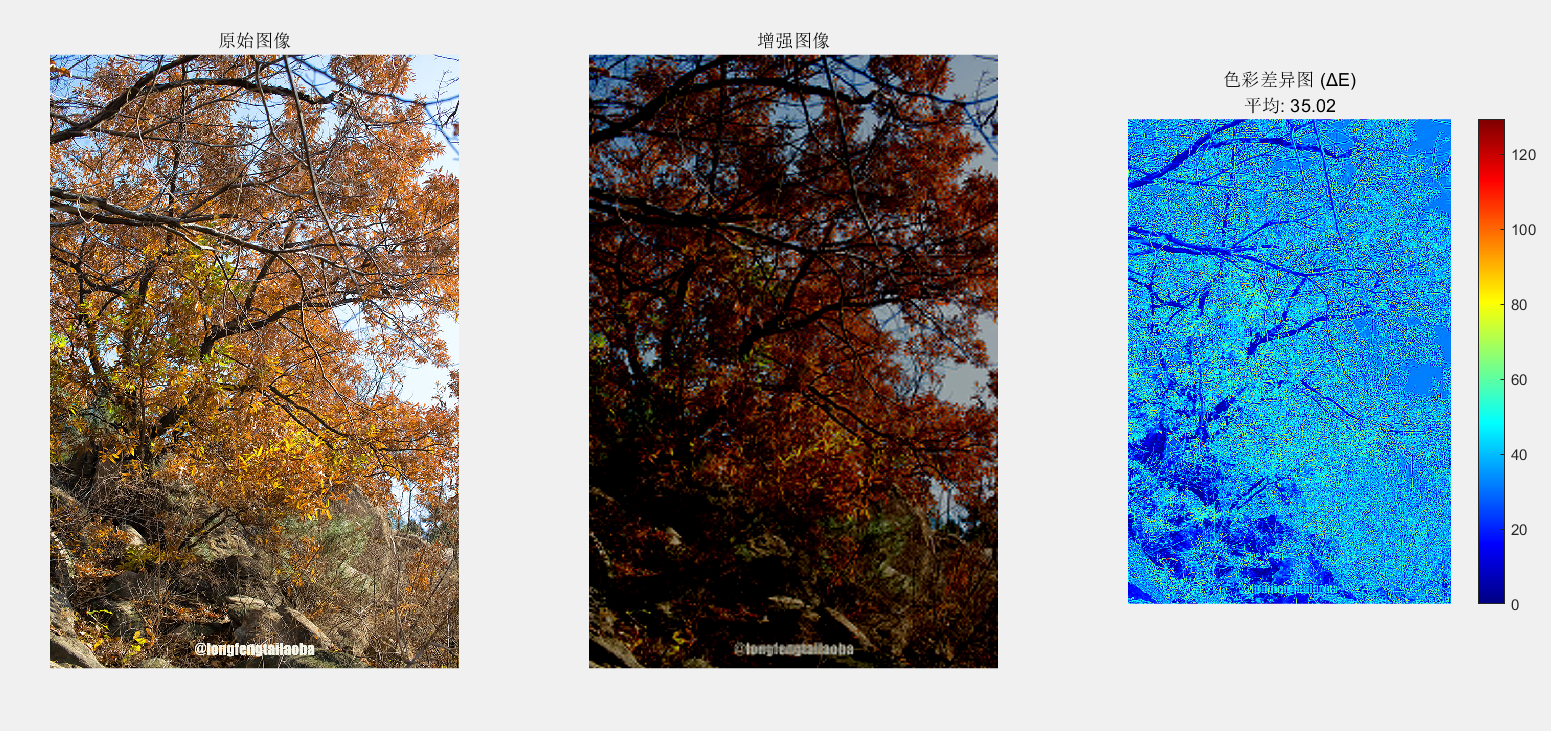
%% 函数3：色彩保持度评估
function color_preservation_eval(original, enhanced, method_name)
    % 评估色彩保持度
    
    % 转换到LAB色彩空间（更适合色彩差异评估）
    original_lab = rgb2lab(original);
    enhanced_lab = rgb2lab(enhanced);
    
    % 计算ΔE（色彩差异）
    delta_E = sqrt(...
        (original_lab(:,:,1) - enhanced_lab(:,:,1)).^2 + ...
        (original_lab(:,:,2) - enhanced_lab(:,:,2)).^2 + ...
        (original_lab(:,:,3) - enhanced_lab(:,:,3)).^2);
    
    mean_deltaE = mean(delta_E(:));
    max_deltaE = max(delta_E(:));
    
    % 计算结构相似性（SSIM）和峰值信噪比（PSNR）
    ssim_val = ssim(rgb2gray(enhanced), rgb2gray(original));
    psnr_val = psnr(enhanced, original);
    
    fprintf('\n%s 方法色彩保持度评估:\n', method_name);
    fprintf('  平均色彩差异 (ΔE): %.2f\n', mean_deltaE);
    fprintf('  最大色彩差异 (ΔE): %.2f\n', max_deltaE);
    fprintf('  结构相似性 (SSIM): %.4f\n', ssim_val);
    fprintf('  峰值信噪比 (PSNR): %.2f dB\n', psnr_val);
    
    % 显示色彩差异图
    figure('Name', ['色彩差异分析 - ', method_name]);
    subplot(1, 3, 1);
    imshow(original);
    title('原始图像');
    
    subplot(1, 3, 2);
    imshow(enhanced);
    title('增强图像');
    
    subplot(1, 3, 3);
    imshow(delta_E, []);
    colormap('jet');
    colorbar;
    title(sprintf('色彩差异图 (ΔE)\n平均: %.2f', mean_deltaE));
end

%% 函数4：批量处理多张图像
function process_image_collection(image_folder, output_folder)
    % 批量处理文件夹中的所有图像
    
    if ~exist(output_folder, 'dir')
        mkdir(output_folder);
    end
    
    % 获取所有图像文件
    image_files = dir(fullfile(image_folder, '*.jpg'));
    image_files = [image_files; dir(fullfile(image_folder, '*.png'))];
    image_files = [image_files; dir(fullfile(image_folder, '*.bmp'))];
    
    fprintf('开始批量处理 %d 张图像...\n', length(image_files));
    
    for i = 1:length(image_files)
        % 读取图像
        img_path = fullfile(image_folder, image_files(i).name);
        img = imread(img_path);
        
        % 仅处理彩色图像
        if size(img, 3) == 3
            % 使用自适应增强
            img_enhanced = adaptive_wavelet_enhance(img);
            
            % 保存结果
            [~, name, ext] = fileparts(image_files(i).name);
            output_path = fullfile(output_folder, [name, '_enhanced', ext]);
            imwrite(img_enhanced, output_path);
            
            fprintf('  已处理: %s\n', image_files(i).name);
        else
            fprintf('  跳过灰度图像: %s\n', image_files(i).name);
        end
    end
    
    fprintf('批量处理完成！\n');
end

%% 函数5：交互式阈值调整界面
function interactive_threshold_adjustment(img_rgb)
    % 创建交互式界面
    
    fig = figure('Name', '交互式阈值调整', ...
                 'Position', [200, 200, 1000, 400]);
    
    % 添加控制面板
    uicontrol('Style', 'text', ...
              'Position', [20, 350, 120, 20], ...
              'String', '阈值因子:');
    
    threshold_slider = uicontrol('Style', 'slider', ...
                                 'Position', [20, 320, 120, 20], ...
                                 'Min', 0.05, 'Max', 0.8, ...
                                 'Value', 0.3, ...
                                 'SliderStep', [0.01, 0.1]);
    
    threshold_text = uicontrol('Style', 'text', ...
                               'Position', [20, 290, 120, 20], ...
                               'String', '0.30');
    
    % 添加颜色空间选择
    uicontrol('Style', 'text', ...
              'Position', [160, 350, 120, 20], ...
              'String', '颜色空间:');
    
    colorspace_popup = uicontrol('Style', 'popupmenu', ...
                                 'Position', [160, 320, 120, 30], ...
                                 'String', {'YCbCr', 'HSV'}, ...
                                 'Value', 1);
    
    % 显示区域
    ax_original = subplot(1, 3, 1);
    imshow(img_rgb);
    title('原始图像');
    
    ax_enhanced = subplot(1, 3, 2);
    
    ax_difference = subplot(1, 3, 3);
    
    % 回调函数
    function update_display(~, ~)
        % 获取当前参数
        threshold_val = threshold_slider.Value;
        colorspace_idx = colorspace_popup.Value;
        
        % 更新显示值
        threshold_text.String = sprintf('%.2f', threshold_val);
        
        % 选择颜色空间
        if colorspace_idx == 1
            colorspace = 'ycbcr';
        else
            colorspace = 'hsv';
        end
        
        % 执行增强
        img_enhanced = wavelet_color_enhance(...
            img_rgb, colorspace, 'sym4', 2, threshold_val);
        
        % 显示增强图像
        axes(ax_enhanced);
        imshow(img_enhanced);
        title(['增强图像\n', ...
               '阈值=', sprintf('%.2f', threshold_val), ...
               ', 空间=', colorspace]);
        
        % 显示差异图
        axes(ax_difference);
        diff_img = imabsdiff(img_rgb, img_enhanced);
        imshow(diff_img * 5); % 放大差异以便观察
        title('增强差异（×5）');
        colorbar;
    end
    
    % 设置回调
    threshold_slider.Callback = @update_display;
    colorspace_popup.Callback = @update_display;
    
    % 初始更新
    update_display();
end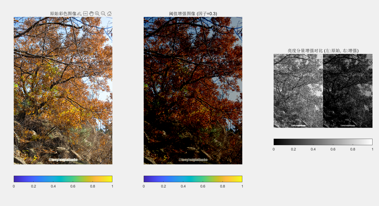

代码说明：

主要功能：

1. 三种增强方法：

   • 细节增强：通过放大高频小波系数来增强图像细节

   • 对比度增强：通过调整低频小波系数来改善对比度

   • 阈值增强：使用软阈值处理去除噪声同时保留细节

2. 小波参数可调：

   • 可选择不同小波基函数（'haar', 'db2', 'sym4'等）

   • 可调整分解层数

   • 可调节增强因子

3. 可视化：

   • 显示原始图像和三种增强结果

   • 显示小波分解的各子带系数

   • 交互式界面调整参数（可选）

使用方法：

1. 将图像文件路径替换为你的图像

2. 调整小波基函数和分解层数

3. 调整增强因子以获得最佳效果

4. 可取消注释第11部分使用交互式界面

注意事项：

• 增强因子需要根据具体图像调整，过大可能导致噪声放大

• 对于彩色图像，建议转换到其他颜色空间（如HSV/YCbCr）后再对亮度分量处理

• 小波基函数选择会影响增强效果，可以尝试不同的小波

这个代码提供了灵活的框架，你可以根据具体需求调整参数或增加其他小波增强算法。