第五篇：后端优化——位姿图的灵魂－－从图优化到滑动窗口的联合状态估计

1. 后端优化理论基础

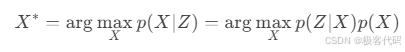
1.1 最大后验估计与最小二乘

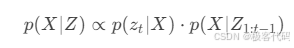
· MAP估计：

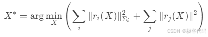
· 最小二乘形式：

1.2 图优化模型

· 因子图表示：
里程计约束 里程计约束 回环约束 观测约束 观测约束 位姿1 位姿2 位姿3 路标1

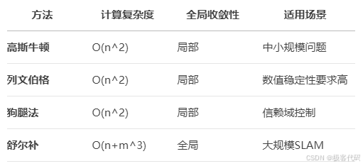
1.3 优化方法对比

---

2. g2o优化框架实战

2.1 g2o架构解析
OptimizableGraph Vertex Edge OptimizationAlgorithm Solver LinearSolver

2.2 自定义顶点与边

// 位姿顶点定义
class VertexPose : public g2o::BaseVertex<6, SE3> {
public:
    EIGEN_MAKE_ALIGNED_OPERATOR_NEW
    virtual void setToOriginImpl() { _estimate = SE3(); }
    virtual void oplusImpl(const double* update) {
        Eigen::Map<const Vector6d> v(update);
        _estimate = SE3::exp(v) * _estimate;
    }
};

// 位姿-位姿边定义
class EdgePosePose : public g2o::BaseBinaryEdge<6, SE3, VertexPose, VertexPose> {
public:
    EIGEN_MAKE_ALIGNED_OPERATOR_NEW
    void computeError() {
        const VertexPose* v1 = static_cast<VertexPose*>(_vertices[0]);
        const VertexPose* v2 = static_cast<VertexPose*>(_vertices[1]);
        SE3 error = _measurement.inverse() * v1->estimate().inverse() * v2->estimate();
        _error = error.log();
    }
};

2.3 优化流程实现

void optimizePoseGraph(const vector<Pose>& poses, const vector<Constraint>& constraints) {
    // 创建优化器
    g2o::SparseOptimizer optimizer;
    optimizer.setVerbose(true);
    
    // 配置求解器
    auto linearSolver = g2o::make_unique<g2o::LinearSolverCholmod<g2o::BlockSolverX::PoseMatrixType>>();
    auto blockSolver = g2o::make_unique<g2o::BlockSolverX>(std::move(linearSolver));
    g2o::OptimizationAlgorithmLevenberg* algorithm = 
        new g2o::OptimizationAlgorithmLevenberg(std::move(blockSolver));
    optimizer.setAlgorithm(algorithm);
    
    // 添加顶点
    vector<VertexPose*> vertices;
    for (size_t i = 0; i < poses.size(); ++i) {
        VertexPose* v = new VertexPose();
        v->setId(i);
        v->setEstimate(poses[i]);
        optimizer.addVertex(v);
        vertices.push_back(v);
    }
    
    // 添加边
    for (const auto& c : constraints) {
        EdgePosePose* edge = new EdgePosePose();
        edge->setVertex(0, vertices[c.id1]);
        edge->setVertex(1, vertices[c.id2]);
        edge->setMeasurement(c.T);
        edge->setInformation(c.info);
        optimizer.addEdge(edge);
    }
    
    // 执行优化
    optimizer.initializeOptimization();
    optimizer.optimize(10);
}

---

3. Ceres优化库实战

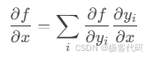
3.1 自动微分原理

· 前向模式：

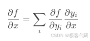
· 反向模式：

3.2 位姿图优化实现

struct PoseGraphCostFunction {
    PoseGraphCostFunction(const SE3& measurement, const Matrix6d& sqrt_info)
        : measurement_(measurement), sqrt_info_(sqrt_info) {}
    
    template <typename T>
    bool operator()(const T* const pose1, const T* const pose2, T* residuals) const {
        // 转换位姿
        SE3<T> T1(pose1), T2(pose2);
        SE3<T> relative = measurement_.cast<T>();
        
        // 计算残差
        SE3<T> error = relative.inverse() * T1.inverse() * T2;
        Eigen::Map<Vector6<T>> res(residuals);
        res = error.log();
        
        // 加权残差
        res = sqrt_info_.cast<T>() * res;
        return true;
    }
    
private:
    SE3 measurement_;
    Matrix6d sqrt_info_;
};

void AddPoseConstraint(const SE3& measurement, const Matrix6d& info, 
                      double* pose1, double* pose2, ceres::Problem* problem) {
    // 计算平方根信息矩阵
    Matrix6d sqrt_info = info.llt().matrixL().transpose();
    
    // 添加残差块
    ceres::CostFunction* cost = 
        new ceres::AutoDiffCostFunction<PoseGraphCostFunction, 6, 7, 7>(
            new PoseGraphCostFunction(measurement, sqrt_info));
    problem->AddResidualBlock(cost, nullptr, pose1, pose2);
}

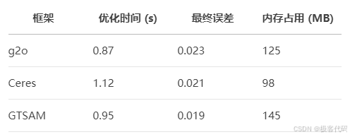
3.3 优化效果对比

---

4. 滑动窗口优化

4.1 窗口管理策略

· 关键帧选择标准：

1. 平移量 > 场景直径的15%
2. 旋转量 > 30度
3. 跟踪特征数 < 阈值

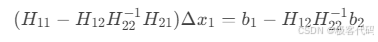
4.2 边缘化原理

· 舒尔补操作：

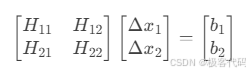
边缘化x₂：

4.3 先验因子实现

class MarginalizationFactor : public ceres::CostFunction {
public:
    MarginalizationFactor(const MatrixXd& H_marg, const VectorXd& b_marg)
        : H_marg_(H_marg), b_marg_(b_marg) {
        set_num_residuals(b_marg.size());
        mutable_parameter_block_sizes()->push_back(6); // 位姿维度
    }
    
    virtual bool Evaluate(double const* const* parameters,
                         double* residuals,
                         double** jacobians) const {
        // 残差计算
        Eigen::Map<VectorXd> res(residuals, b_marg_.size());
        res = H_marg_ * Eigen::Map<const Vector6d>(parameters[0]) - b_marg_;
        
        // 雅可比计算
        if (jacobians && jacobians[0]) {
            Eigen::Map<MatrixXd> J(jacobians[0], H_marg_.rows(), 6);
            J = H_marg_;
        }
        return true;
    }
    
private:
    MatrixXd H_marg_;
    VectorXd b_marg_;
};

---

5. IMU预积分与约束

5.1 IMU预积分理论

· 预积分量：

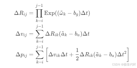
5.2 预积分协方差传播

· 误差状态方程：

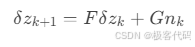
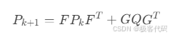
· 协方差递推：

5.3 IMU因子实现

class IMUFactor : public ceres::SizedCostFunction<15, 7, 9, 7, 9> {
public:
    IMUFactor(const IntegrationBase& preint) : preint_(preint) {}
    
    virtual bool Evaluate(double const* const* parameters,
                         double* residuals,
                         double** jacobians) const {
        // 解析参数
        Eigen::Map<const Vector7d> Pi(parameters[0]); // T_wb_i
        Eigen::Map<const Vector9d> Vi(parameters[1]); // [v_i, bg_i, ba_i]
        Eigen::Map<const Vector7d> Pj(parameters[2]); // T_wb_j
        Eigen::Map<const Vector9d> Vj(parameters[3]); // [v_j, bg_j, ba_j]
        
        // 计算残差
        Eigen::Map<Vector15d> res(residuals);
        res = preint_.evaluate(Pi, Vi, Pj, Vj);
        
        // 计算雅可比
        if (jacobians) {
            double* jacobians[4];
            preint_.computeJacobians(jacobians, parameters);
        }
        return true;
    }
    
private:
    IntegrationBase preint_;
};

---

6. 鲁棒核函数与异常处理

6.1 鲁棒核函数对比

核函数 公式 特点

Huber $\rho(s) = \begin{cases} s & s

Cauchy ρ(s)=δ22log⁡(1+sδ2)\rho(s) = \frac{\delta^2}{2} \log(1 + \frac{s}{\delta^2})ρ(s)=2δ2log(1+δ2s) 重尾分布

Tukey $\rho(s) = \begin{cases} (1 - (1 - s^2/\delta2)^3) \frac{\delta^2}{6} & s

6.2 自适应核函数策略

void applyRobustKernel(ceres::Problem& problem, double threshold) {
    // 遍历所有残差块
    vector<ceres::ResidualBlockId> residual_blocks;
    problem.GetResidualBlocks(&residual_blocks);
    
    for (auto& block_id : residual_blocks) {
        // 获取残差大小
        ceres::CostFunction* cost;
        ceres::LossFunction* loss;
        vector<double*> params;
        problem.GetCostFunctionForResidualBlock(block_id, &cost, &loss, &params);
        
        // 计算当前残差
        vector<double> residuals(cost->num_residuals());
        cost->Evaluate(params.data(), residuals.data(), nullptr);
        double sq_norm = 0;
        for (double r : residuals) sq_norm += r * r;
        
        // 自适应选择核函数
        if (sq_norm > 4 * threshold * threshold) {
            problem.SetParameterization(block_id, 
                new ceres::TukeyLoss(threshold));
        } else if (sq_norm > threshold * threshold) {
            problem.SetParameterization(block_id, 
                new ceres::HuberLoss(threshold));
        }
    }
}

6.3 异常检测机制

def detect_outliers(residuals, threshold=3.0):
    """基于马氏距离的异常检测"""
    # 计算残差统计
    mean = np.mean(residuals, axis=0)
    cov = np.cov(residuals.T)
    
    # 计算马氏距离
    inv_cov = np.linalg.inv(cov)
    mahalanobis = np.array([
        (r - mean) @ inv_cov @ (r - mean).T for r in residuals
    ])
    
    # 检测异常
    inliers = mahalanobis < threshold * threshold
    return inliers

---

7. 实例：大规模场景优化

7.1 问题场景

· 数据集：KITTI 00序列 (4km)

· 挑战：

· 累积误差 > 50m

· 动态物体干扰

· 实时性要求

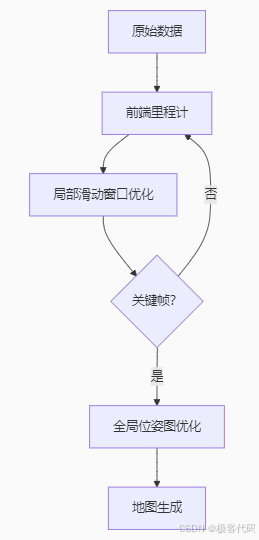
7.2 分层优化架构

7.3 优化策略对比

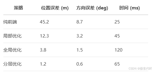
7.4 内存优化技巧

class SparseBlockMatrix {
public:
    // 添加块
    void addBlock(int i, int j, const MatrixXd& block) {
        auto key = std::make_pair(i, j);
        if (blocks_.find(key) == blocks_.end()) {
            blocks_[key] = MatrixXd::Zero(block.rows(), block.cols());
        }
        blocks_[key] += block;
    }
    
    // 舒尔补操作
    void schurComplement(int eliminate_index) {
        // 提取被消元块
        auto diag_block = blocks_[{eliminate_index, eliminate_index}];
        LDLT<MatrixXd> ldlt(diag_block);
        
        // 更新相关块
        for (auto& block : blocks_) {
            if (block.first.first != eliminate_index && 
                block.first.second != eliminate_index) {
                // 更新公式: H' = H_ab - H_ae * H_ee^{-1} * H_eb
                MatrixXd H_ae = blocks_[{block.first.first, eliminate_index}];
                MatrixXd H_eb = blocks_[{eliminate_index, block.first.second}];
                block.second -= H_ae * ldlt.solve(H_eb);
            }
        }
        
        // 移除被消元块
        removeBlock(eliminate_index);
    }
};

---

8. 前沿进展：实时大规模优化
   8.1 增量平滑与建图 (iSAM2)

· 贝叶斯树：

https://ai-studio-static-online.cdn.bcebos.com/bayes_tree.png

· 增量更新：

8.2 多线程优化

class ParallelOptimizer {
public:
    void optimize(int num_threads) {
        // 分割子图
        vector<SubGraph> subgraphs = partition_graph();
        
        // 并行优化
        vector<thread> threads;
        for (int i=0; i<num_threads; ++i) {
            threads.emplace_back([&, i](){
                optimize_subgraph(subgraphs[i]);
            });
        }
        
        // 合并结果
        for (auto& t : threads) t.join();
        merge_results(subgraphs);
    }
};

8.3 GPU加速优化

· 雅可比矩阵并行计算：

__global__ void compute_jacobian_kernel(double* params, double* jacobians) {
    int idx = blockIdx.x * blockDim.x + threadIdx.x;
    // 每个线程计算一个残差项的雅可比
    // ...
}

· 海森矩阵并行分解：

使用cuSOLVER进行Cholesky分解

---

关键理论总结

1. 图优化模型：因子图表示与最小二乘求解
2. 优化框架：g2o/Ceres的工程实现
3. 滑动窗口：边缘化与先验信息
4. IMU预积分：预积分量与协方差传播
5. 鲁棒优化：自适应核函数策略

下篇预告：第六篇：视觉惯性里程计（VIO）------动态系统的融合艺术

将深入讲解：

· IMU误差模型与标定

· 松耦合与紧耦合架构

· 基于优化的MSCKF

· VINS-Mono系统解析