文章目录
1、numpy
1.1、np.where
python
x = np.array([[1, 2], [3, 4]])
print(np.where(x > 2, True, False))
python
# 打印结果
[[False False]
 [ True  True]]
1.2、@运算
python
# 2D X 2D
A = np.random.rand(3, 4)
B = np.random.rand(4, 5)
C = A @ B
print("2D X 2D:", A.shape, "X", B.shape, "=", C.shape)

# 3D X 3D
A = np.random.rand(10, 3, 4)
B = np.random.rand(10, 4, 5)
C = A @ B
print("3D X 3D:", A.shape, "X", B.shape, "=", C.shape)

# 3D X 4D
A = np.random.rand(2, 3, 4)      # shape (2, 3, 4) → 3D
B = np.random.rand(5, 2, 4, 6)   # shape (5, 2, 4, 6) → 4D
# 要求:A.shape[-1] == B.shape[-2]
C = A @ B
print("3D X 4D:", A.shape, "X", B.shape, "=", C.shape)

# 3D X 4D
A = np.random.rand(1, 3, 4)      # shape (2, 3, 4) → 3D
B = np.random.rand(5, 2, 4, 6)   # shape (5, 2, 4, 6) → 4D
# 要求:A.shape[-1] == B.shape[-2]
C = A @ B
print("3D X 4D:", A.shape, "X", B.shape, "=", C.shape)

# 3D X 4D
A = np.random.rand(2, 3, 4)      # shape (2, 3, 4) → 3D
B = np.random.rand(5, 1, 4, 6)   # shape (5, 2, 4, 6) → 4D
# 要求:A.shape[-1] == B.shape[-2]
C = A @ B
print("3D X 4D:", A.shape, "X", B.shape, "=", C.shape)

# 4D X 3D
A = np.random.rand(5, 3, 4, 6)   # shape (5, 2, 4, 6) → 4D
B = np.random.rand(3, 6, 4)      # shape (2, 3, 4) → 3D
# 要求:A.shape[-1] == B.shape[-2]
C = A @ B
print("4D X 3D:", A.shape, "X", B.shape, "=", C.shape)

# 4D X 3D
A = np.random.rand(5, 1, 4, 6)   # shape (5, 2, 4, 6) → 4D
B = np.random.rand(3, 6, 4)      # shape (2, 3, 4) → 3D
# 要求:A.shape[-1] == B.shape[-2]
C = A @ B
print("4D X 3D:", A.shape, "X", B.shape, "=", C.shape)

# 4D X 3D
A = np.random.rand(5, 3, 4, 6)   # shape (5, 2, 4, 6) → 4D
B = np.random.rand(1, 6, 4)      # shape (2, 3, 4) → 3D
# 要求:A.shape[-1] == B.shape[-2]
C = A @ B
print("4D X 3D:", A.shape, "X", B.shape, "=", C.shape)

# 3D X 4D
A = np.random.rand(3, 3, 4)      # shape (2, 3, 4) → 3D
B = np.random.rand(5, 2, 4, 6)   # shape (5, 2, 4, 6) → 4D
# 要求:A.shape[-1] == B.shape[-2]
try:
    C = A @ B
    print("3D X 4D:", A.shape, "X", B.shape, "=", C.shape)
except ValueError as e:
    print("❌ 3D X 4D 失败!")
    print("   提示:A.shape[-1] == B.shape[-2]")
    print("        确保批处理维度可以广播。")
    print("   广播规则1:广播从右向左对齐, 不包括最后两维")
    print("   广播规则2:维度要么相等,要么其中一个是 1,否则报错")
    print("   详细错误:", e)

# 4D X 3D
A = np.random.rand(5, 3, 4, 6)   # shape (5, 2, 4, 6) → 4D
B = np.random.rand(2, 6, 4)      # shape (2, 3, 4) → 3D
# 要求:A.shape[-1] == B.shape[-2]
try:
    C = A @ B
    print("3D X 4D:", A.shape, "X", B.shape, "=", C.shape)
except ValueError as e:
    print("❌ 4D X 3D 失败!")
    print("   提示:A.shape[-1] == B.shape[-2]")
    print("        确保批处理维度可以广播。")
    print("   广播规则1:广播从右向左对齐, 不包括最后两维")
    print("   广播规则2:维度要么相等,要么其中一个是 1,否则报错")
    print("   详细错误:", e)
bash
# 打印结果
2D X 2D: (3, 4) X (4, 5) = (3, 5)
3D X 3D: (10, 3, 4) X (10, 4, 5) = (10, 3, 5)
3D X 4D: (2, 3, 4) X (5, 2, 4, 6) = (5, 2, 3, 6)
3D X 4D: (1, 3, 4) X (5, 2, 4, 6) = (5, 2, 3, 6)
3D X 4D: (2, 3, 4) X (5, 1, 4, 6) = (5, 2, 3, 6)
4D X 3D: (5, 3, 4, 6) X (3, 6, 4) = (5, 3, 4, 4)
4D X 3D: (5, 1, 4, 6) X (3, 6, 4) = (5, 3, 4, 4)
4D X 3D: (5, 3, 4, 6) X (1, 6, 4) = (5, 3, 4, 4)
❌ 3D X 4D 失败!
   提示:A.shape[-1] == B.shape[-2]
        确保批处理维度可以广播。
   广播规则1:广播从右向左对齐, 不包括最后两维
   广播规则2:维度要么相等,要么其中一个是 1,否则报错
   详细错误: operands could not be broadcast together with remapped shapes [original->remapped]: (3,3,4)->(3,newaxis,newaxis) (5,2,4,6)->(5,2,newaxis,newaxis)  and requested shape (3,6)
❌ 4D X 3D 失败!
   提示:A.shape[-1] == B.shape[-2]
        确保批处理维度可以广播。
   广播规则1:广播从右向左对齐, 不包括最后两维
   广播规则2:维度要么相等,要么其中一个是 1,否则报错
   详细错误: operands could not be broadcast together with remapped shapes [original->remapped]: (5,3,4,6)->(5,3,newaxis,newaxis) (2,6,4)->(2,newaxis,newaxis)  and requested shape (4,4)
1.3、np.arange
python
np.arange(0,10)
np.arange(0,10,2)
bash
# 打印结果
array([0, 1, 2, 3, 4, 5, 6, 7, 8, 9])
array([0, 2, 4, 6, 8])
1.4、随机数生
1.4.1、随机数生成
python
# 正太分布
np.random.normal(loc=[6, 2.5], scale=[0.5, 0.5], size=(50, 2)).shape
# 标准正太分布
np.random.rand(50,2).shape
bash
# 打印结果
(50, 2)
(50, 2)
1.4.2、随机种子
python
rgen = np.random.RandomState(666)
rgen.normal(loc=[5, 1], scale=[0.5, 0.5], size=(50, 2)).shape
bash
# 打印结果
(50, 2)
或者
python
np.random.seed(0)
np.random.normal(loc=[5, 1], scale=[0.5, 0.5], size=(50, 2)).shape
bash
# 打印结果
(50, 2)
1.5、矩阵拼接
1.5.1、np.vstack
拼接第0维,其余维度要完全一致
python
x = np.random.rand(9,2,3,4)
y = np.random.rand(2,2,3,4)
np.vstack((y,x)).shape
bash
# 打印结果
(11, 2, 3, 4)
1.5.2、np.hstack
拼接第1维,其余维度要完全一致
python
x = np.random.rand(66,9,2,3,4)
y = np.random.rand(66,3,2,3,4)
np.hstack((y,x)).shape
bash
# 打印结果
(66, 12, 2, 3, 4)
1.5.3、np.concatenate
拼接指定的axis维,除了axis维,其余维度要完全一致
python
x = np.random.rand(9,2,1,4)
y = np.random.rand(9,2,3,4)
np.concatenate((x,y), axis=2).shape
bash
# 打印结果
(9, 2, 4, 4)
1.5.4、np.stack
把多个形状相同的数组,沿着一个新轴axis堆叠起来,形成更高维的数组。
| axis | 输出形状 | 含义 |
|---|---|---|
| 0 | (N, 1, 2, 3, 4) |
在最前面加一维 |
| 1 | (1, N, 2, 3, 4) |
|
| 2 | (1, 2, N, 3, 4) |
|
| 3 | (1, 2, 3, N, 4) |
|
| 4 | (1, 2, 3, 4, N) |
在最后面加一维 |
python
a = np.random.rand(1,2,3,4)
b = np.random.rand(1,2,3,4)
print(np.stack((a, b), axis=0).shape)
print(np.stack((a, b), axis=1).shape)
print(np.stack((a, b), axis=2).shape)
print(np.stack((a, b), axis=3).shape)
print(np.stack((a, b), axis=4).shape)
bash
# 打印结果
(2, 1, 2, 3, 4)
(1, 2, 2, 3, 4)
(1, 2, 2, 3, 4)
(1, 2, 3, 2, 4)
(1, 2, 3, 4, 2)
2、pytorch
3、matplotlib
3.1、散点图
python
import numpy as np
import matplotlib.pyplot as plt

# 设置随机种子以便结果可复现
np.random.seed(0)

# 生成第一组数据(模拟'Iris-setosa')
# (50,2)
data_setosa = np.random.normal(loc=[5, 1], scale=[0.5, 0.5], size=(50, 2))

# 生成第二组数据(模拟'Versicolor')
# (50,2)
data_versicolor = np.random.normal(loc=[6, 2.5], scale=[0.5, 0.5], size=(50, 2))

# 合并数据
# (100,2)
x = np.vstack((data_setosa, data_versicolor))

# 创建标签
# (100,)
y = np.hstack((np.zeros(50), np.ones(50)))

# 绘制散点图
plt.scatter(x[:50, 0], x[:50, 1], color='red', marker='o', label='Simulated Setosa')
plt.scatter(x[50:100, 0], x[50:100, 1], color='green', marker='s', label='Simulated Versicolor')

# 添加轴标签和图例
plt.xlabel('Feature 1')
plt.ylabel('Feature 2')
plt.legend(loc='upper left')

# 显示图形
plt.show()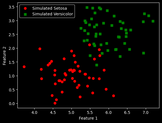
3.2、多张图
1行2列个子图
python
import numpy as np
import matplotlib.pyplot as plt

# 随机生成数据
np.random.seed(0)  # 确保结果可复现
losses_ada1 = np.random.rand(10)  # 学习率0.1的损失值
losses_ada2 = np.random.rand(10)  # 学习率0.0001的损失值

# 创建1行2列的子图
fig, ax = plt.subplots(nrows=1, ncols=2, figsize=(10, 4))

# 第一个子图:学习率0.1
ax[0].plot(range(1, len(losses_ada1) + 1), losses_ada1, marker='o')
ax[0].set_xlabel('Epochs')
ax[0].set_ylabel('Loss')
ax[0].set_title('Adaline - Learning rate 0.1')

# 第二个子图:学习率0.0001
ax[1].plot(range(1, len(losses_ada2) + 1), losses_ada2, marker='o')
ax[1].set_xlabel('Epochs')
ax[1].set_ylabel('Loss')
ax[1].set_title('Adaline - Learning rate 0.0001')

# 显示图形
plt.show()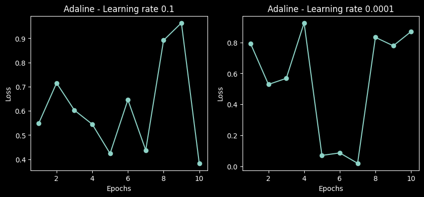
3.3、热力图
python
import numpy as np
import matplotlib.pyplot as plt

# 1. 创建 x 和 y 的一维坐标
x = np.linspace(-2, 2, 100)   # 从 -2 到 2,取 100 个点
y = np.linspace(-2, 2, 100)

# 2. 生成网格(每个点都有 (x, y) 坐标)
X, Y = np.meshgrid(x, y)

# 3. 定义一个函数:比如到原点的距离(形成圆形等高线)
Z = np.sqrt(X**2 + Y**2)   # 每个网格点到 (0,0) 的距离

# 4. 用 contourf 填充颜色
plt.contourf(X, Y, Z, levels=20, cmap='viridis')

# 5. 添加颜色条(可选)
plt.colorbar(label='Distance from origin')

# 6. 设置标题和坐标轴
plt.title('Demo: plt.contourf')
plt.xlabel('X')
plt.ylabel('Y')

# 7. 显示图形
plt.show()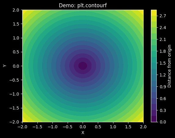
4、scikit-learn
4.1、train_test_split(划分:训练集、测试集)
参数stratify:确保训练集和测试集中,每个类别样本的比例与划分前的数据集一致
python
from sklearn import datasets
import numpy as np
from sklearn.model_selection import train_test_split

iris = datasets.load_iris()
X = iris.data[:, [2, 3]]
y = iris.target

X_train, X_test, y_train, y_test = train_test_split(
    X, y, test_size=0.3, random_state=1, stratify=y)

print('Labels counts in y:', np.bincount(y))
print('Labels counts in y_train:', np.bincount(y_train))
print('Labels counts in y_test:', np.bincount(y_test))
bash
Labels counts in y: [50 50 50]
Labels counts in y_train: [35 35 35]
Labels counts in y_test: [15 15 15]
4.2、StratifiedKFold(交叉验证,划分:训练集、测试集)
python
from sklearn.model_selection import StratifiedKFold
from sklearn import datasets
import numpy as np

iris = datasets.load_iris()
X, y = iris.data, iris.target

skf = StratifiedKFold(n_splits=5, shuffle=True)  # 不打乱,便于观察

for fold, (train_idx, val_idx) in enumerate(skf.split(X, y), 1):
    print(f"Fold {fold}:")
    print("  训练集类别分布:", np.bincount(y[train_idx]))
    print("  验证集类别分布:", np.bincount(y[val_idx]))
bash
Fold 1:
  训练集类别分布: [40 40 40]
  验证集类别分布: [10 10 10]
Fold 2:
  训练集类别分布: [40 40 40]
  验证集类别分布: [10 10 10]
Fold 3:
  训练集类别分布: [40 40 40]
  验证集类别分布: [10 10 10]
Fold 4:
  训练集类别分布: [40 40 40]
  验证集类别分布: [10 10 10]
Fold 5:
  训练集类别分布: [40 40 40]
  验证集类别分布: [10 10 10]
4.3、accuracy_score(计算ACC)
python
from sklearn.metrics import accuracy_score

print('Accuracy: %.3f' % accuracy_score(y_test, y_pred))
实践
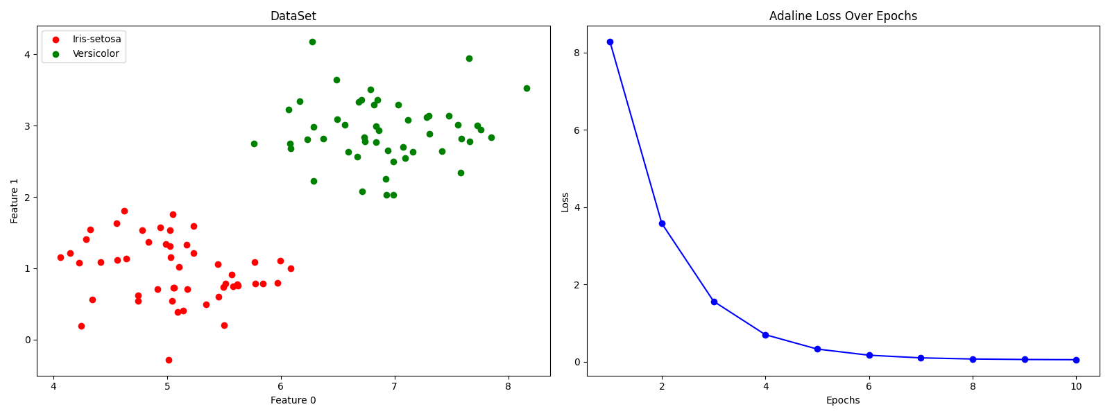
实践1:简单二分类
python
import numpy as np
import matplotlib.pyplot as plt

# load data
x1 = np.random.normal(loc=[5, 1], scale=[0.5,0.5], size=(50,2))
x2 = np.random.normal(loc=[7, 3], scale=[0.5,0.5], size=(50,2))
x = np.vstack((x1,x2))
y = np.hstack((np.zeros(50), np.ones(50)))

# plot data and loss in subplots
fig, (ax1, ax2) = plt.subplots(1, 2, figsize=(16, 6))

# scatter plot of the data points
ax1.scatter(x[:50, 0], x[:50, 1], color='red', marker='o', label='Iris-setosa')
ax1.scatter(x[50:100, 0], x[50:100, 1], color='green', marker='o', label='Versicolor')
ax1.set_xlabel('Feature 0')
ax1.set_ylabel('Feature 1')
ax1.set_title('DataSet')
ax1.legend(loc='upper left')

# model
class AdalineSGD:
    def __init__(self, epochs=10, lr=0.0001, seed=6):
        self.epochs = epochs
        self.lr = lr
        self.rgen = np.random.RandomState(seed)
        self.loss = []

    def init_params(self, shape):
        self.w_ = self.rgen.normal(loc=0.5, scale=0.05, size=shape)
        self.b_ = np.float_(0.0)

    def update_params(self, xi, yi):
        out = self.activate(self.net_input(xi))
        error = yi - out
        self.w_ += self.lr * error * xi
        self.b_ += self.lr * error
        return error ** 2

    def shuffle(self, x, y):
        r = self.rgen.permutation(len(y))
        return x[r], y[r]

    def fit(self, x, y):
        self.init_params(x.shape[1])
        x, y = self.shuffle(x, y)
        for _ in range(self.epochs):
            loss = []
            for xi, yi in zip(x, y):
                loss.append(self.update_params(xi, yi))
            self.loss.append(np.mean(loss))

    def net_input(self, x):
        return x @ self.w_ + self.b_

    def activate(self, x):
        return x

    def predict(self, x):
        return np.where(self.activate(self.net_input(x)) >= 0.5, 0, 1)

model = AdalineSGD()
model.fit(x, y)

# plot loss over epochs
ax2.plot(np.arange(1, len(model.loss) + 1), model.loss, color='blue', marker='o')
ax2.set_xlabel('Epochs')
ax2.set_ylabel('Loss')
ax2.set_title('Adaline Loss Over Epochs')

plt.tight_layout()
plt.show()