摘要
本文将深入探讨数字滤波器的各种基本结构,包括IIR和FIR滤波器的不同实现方式。通过理论讲解、MATLAB代码实现和可视化对比,帮助读者全面理解数字滤波器的结构特点及应用。
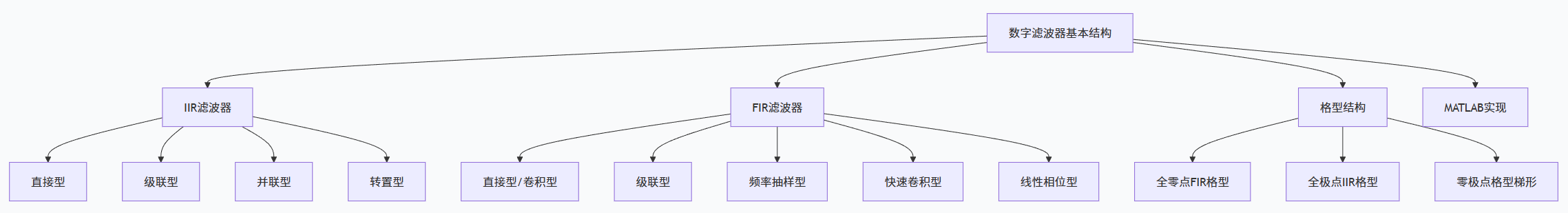
目录结构
5.1 概述
数字滤波器是数字信号处理中的核心组件,其基本结构决定了滤波器的性能和实现复杂度。本章将系统讲解IIR和FIR滤波器的各种实现结构。
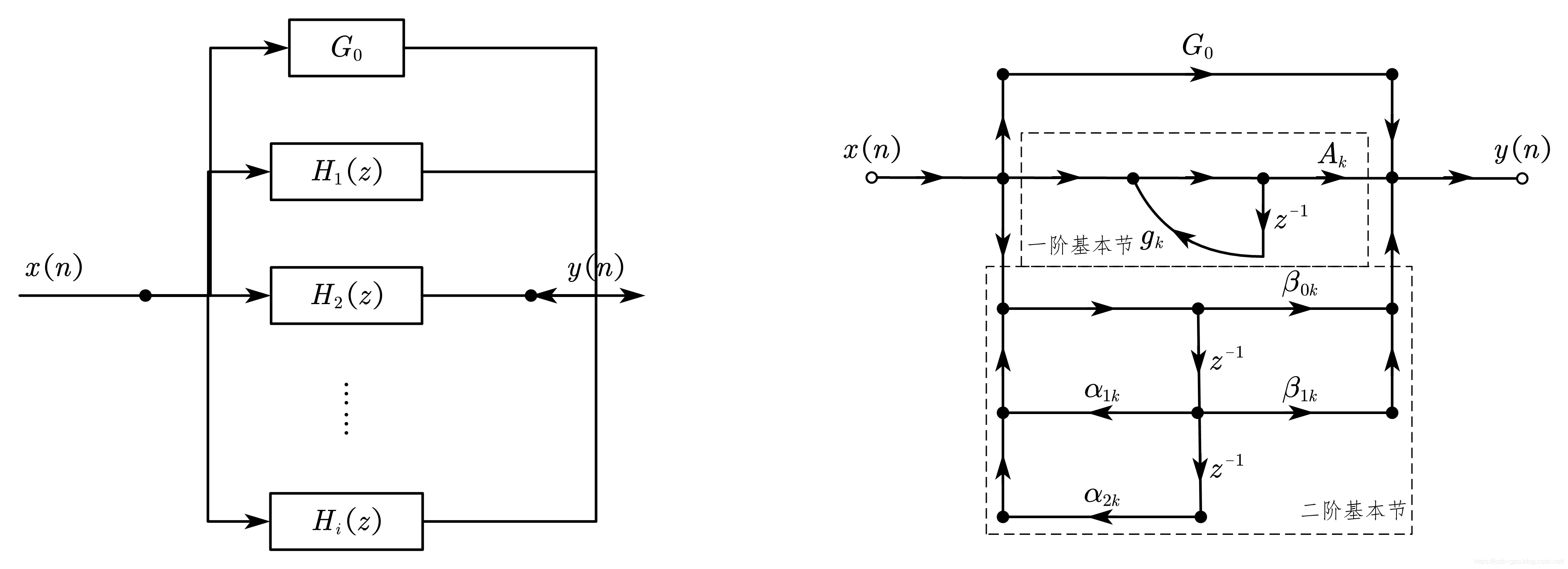
5.2 无限长单位冲激响应(IIR)滤波器的基本结构
5.2.1 IIR滤波器的特点
IIR滤波器具有递归结构,系统函数同时包含零点和极点,通常用差分方程表示:
y(n) = Σb_k·x(n-k) - Σa_k·y(n-k) (k=0 to M, a_0=1)
5.2.2 直接型结构
直接型结构是IIR滤波器最直观的实现方式,分为直接Ⅰ型和直接Ⅱ型。
Matlab
%% 5.2.2 IIR直接型滤波器实现与比较
% 清理环境
clear; close all; clc;

% 生成测试信号:包含10Hz、50Hz和100Hz的正弦波
fs = 500;           % 采样频率
t = 0:1/fs:1;       % 时间向量
f1 = 10; f2 = 50; f3 = 100; % 频率成分

% 合成信号
x = sin(2*pi*f1*t) + 0.5*sin(2*pi*f2*t) + 0.3*sin(2*pi*f3*t);
x = x + 0.1*randn(size(t)); % 添加噪声

% 设计一个4阶带阻IIR滤波器,阻带45-55Hz
fc1 = 45/(fs/2);    % 归一化下截止频率
fc2 = 55/(fs/2);    % 归一化上截止频率
[b, a] = butter(2, [fc1, fc2], 'stop'); % 2阶巴特沃斯带阻滤波器

% 直接型滤波实现
y_direct = filter(b, a, x);

% 可视化对比
figure('Position', [100, 100, 1200, 800]);

% 原始信号时域
subplot(3, 2, 1);
plot(t, x, 'b', 'LineWidth', 1.5);
title('原始信号 (时域)', 'FontSize', 12, 'FontWeight', 'bold');
xlabel('时间 (s)'); ylabel('幅度');
grid on; xlim([0, 0.5]);

% 原始信号频域
subplot(3, 2, 2);
N = length(x);
X = fft(x, N);
f = (0:N-1)*(fs/N);
plot(f(1:N/2), abs(X(1:N/2)), 'b', 'LineWidth', 1.5);
title('原始信号频谱', 'FontSize', 12, 'FontWeight', 'bold');
xlabel('频率 (Hz)'); ylabel('幅度');
grid on; xlim([0, 150]);

% 滤波后信号时域
subplot(3, 2, 3);
plot(t, y_direct, 'r', 'LineWidth', 1.5);
title('直接型滤波后信号 (时域)', 'FontSize', 12, 'FontWeight', 'bold');
xlabel('时间 (s)'); ylabel('幅度');
grid on; xlim([0, 0.5]);

% 滤波后信号频域
subplot(3, 2, 4);
Y = fft(y_direct, N);
plot(f(1:N/2), abs(Y(1:N/2)), 'r', 'LineWidth', 1.5);
title('滤波后信号频谱', 'FontSize', 12, 'FontWeight', 'bold');
xlabel('频率 (Hz)'); ylabel('幅度');
grid on; xlim([0, 150]);

% 滤波器频率响应
subplot(3, 2, [5, 6]);
[h, w] = freqz(b, a, 1024, fs);
plot(w, 20*log10(abs(h)), 'g', 'LineWidth', 2);
title('IIR带阻滤波器频率响应', 'FontSize', 12, 'FontWeight', 'bold');
xlabel('频率 (Hz)'); ylabel('幅度 (dB)');
grid on; xlim([0, 150]);
hold on;
% 标记阻带区域
fill([45, 45, 55, 55], [-100, 0, 0, -100], 'r', 'FaceAlpha', 0.2, 'EdgeColor', 'none');
legend('频率响应', '阻带(45-55Hz)', 'Location', 'best');

sgtitle('IIR直接型滤波器效果对比', 'FontSize', 14, 'FontWeight', 'bold');

% 显示滤波器系数
fprintf('IIR直接型滤波器系数:\n');
fprintf('分子系数 b: '); fprintf('%.4f ', b); fprintf('\n');
fprintf('分母系数 a: '); fprintf('%.4f ', a); fprintf('\n');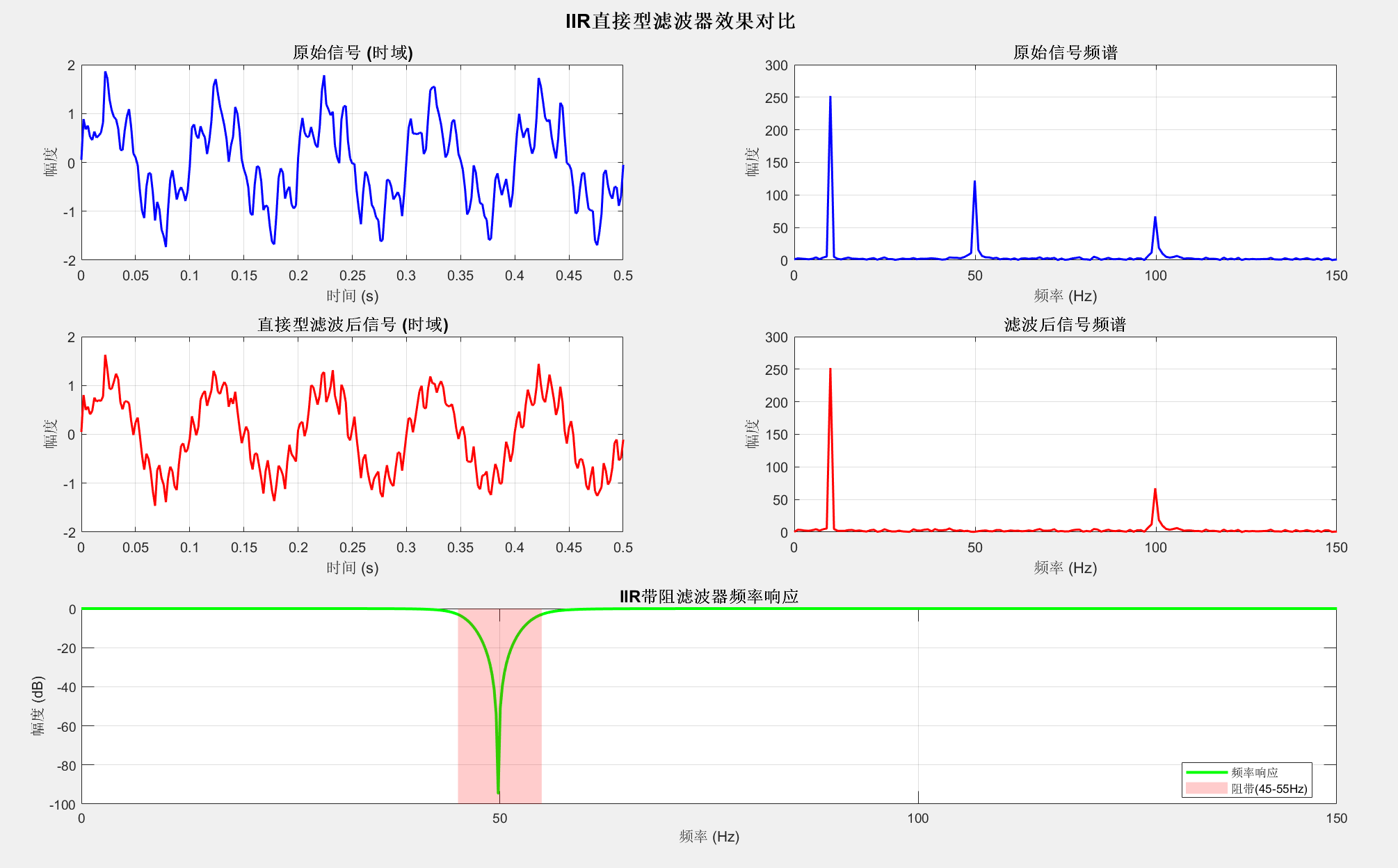
5.2.3 级联型结构
级联型将高阶滤波器分解为多个二阶节的级联,提高了数值稳定性。
Matlab
%% 5.2.3 IIR级联型结构实现

% 清理环境

clear; close all; clc;


% 生成测试信号:包含多种频率成分的合成信号

fs = 1000; % 采样频率

t = 0:1/fs:2; % 时间向量(2秒)

N = length(t); % 信号长度


% 生成多频率信号

x = zeros(size(t));

frequencies = [20, 80, 150, 220, 300]; % 多个频率成分

amplitudes = [1, 0.7, 0.5, 0.3, 0.2]; % 对应幅度


for i = 1:length(frequencies)

x = x + amplitudes(i) * sin(2*pi*frequencies(i)*t);

end


% 添加噪声

x = x + 0.15*randn(size(t));


% 设计一个6阶IIR低通滤波器,截止频率100Hz

fc = 100/(fs/2); % 归一化截止频率

[b, a] = butter(6, fc, 'low'); % 6阶巴特沃斯低通滤波器


% 将高阶滤波器分解为二阶节(SOS:Second-Order Sections)

[sos, g] = tf2sos(b, a);

num_sections = size(sos, 1); % 二阶节的数量


fprintf('级联型结构:将6阶滤波器分解为%d个二阶节\n', num_sections);

disp('每个二阶节的系数矩阵(每行: [b0, b1, b2, 1, a1, a2]):');

disp(sos);

fprintf('增益系数 g: %.6f\n', g);


% 级联型滤波实现

y_cascade = x * g; % 先乘整体增益


% 对每个二阶节进行滤波

for i = 1:num_sections

b_section = sos(i, 1:3); % 当前二阶节的分子系数

a_section = sos(i, 4:6); % 当前二阶节的分母系数

y_cascade = filter(b_section, a_section, y_cascade);

end


% 直接型滤波作为对比

y_direct = filter(b, a, x);


% 可视化对比

figure('Position', [100, 100, 1400, 800]);


% 原始信号

subplot(3, 3, 1);

plot(t, x, 'b', 'LineWidth', 1.2);

title('原始信号', 'FontSize', 11, 'FontWeight', 'bold');

xlabel('时间 (s)'); ylabel('幅度');

grid on; xlim([0, 0.5]);


% 原始信号频谱

subplot(3, 3, 2);

X = fft(x, N);

f = (0:N-1)*(fs/N);

plot(f(1:N/2), abs(X(1:N/2)), 'b', 'LineWidth', 1.2);

title('原始信号频谱', 'FontSize', 11, 'FontWeight', 'bold');

xlabel('频率 (Hz)'); ylabel('幅度');

grid on; xlim([0, 400]);


% 滤波器频率响应

subplot(3, 3, 3);

[h, w] = freqz(b, a, 1024, fs);

plot(w, 20*log10(abs(h)), 'k', 'LineWidth', 2);

title('6阶低通滤波器频率响应 (fc=100Hz)', 'FontSize', 11, 'FontWeight', 'bold');

xlabel('频率 (Hz)'); ylabel('幅度 (dB)');

grid on; xlim([0, 400]);

hold on;

plot([100, 100], [-60, 0], 'r--', 'LineWidth', 1.5);

legend('频率响应', '截止频率', 'Location', 'best');


% 直接型滤波结果

subplot(3, 3, 4);

plot(t, y_direct, 'r', 'LineWidth', 1.2);

title('直接型滤波结果', 'FontSize', 11, 'FontWeight', 'bold');

xlabel('时间 (s)'); ylabel('幅度');

grid on; xlim([0, 0.5]);


subplot(3, 3, 5);

Y_direct = fft(y_direct, N);

plot(f(1:N/2), abs(Y_direct(1:N/2)), 'r', 'LineWidth', 1.2);

title('直接型滤波频谱', 'FontSize', 11, 'FontWeight', 'bold');

xlabel('频率 (Hz)'); ylabel('幅度');

grid on; xlim([0, 400]);


% 级联型滤波结果

subplot(3, 3, 7);

plot(t, y_cascade, 'g', 'LineWidth', 1.2);

title('级联型滤波结果', 'FontSize', 11, 'FontWeight', 'bold');

xlabel('时间 (s)'); ylabel('幅度');

grid on; xlim([0, 0.5]);


subplot(3, 3, 8);

Y_cascade = fft(y_cascade, N);

plot(f(1:N/2), abs(Y_cascade(1:N/2)), 'g', 'LineWidth', 1.2);

title('级联型滤波频谱', 'FontSize', 11, 'FontWeight', 'bold');

xlabel('频率 (Hz)'); ylabel('幅度');

grid on; xlim([0, 400]);


% 两种结构结果对比

subplot(3, 3, [6, 9]);

plot(t(1:500), y_direct(1:500), 'r', 'LineWidth', 1.5);

hold on;

plot(t(1:500), y_cascade(1:500), 'g--', 'LineWidth', 1.5);

title('直接型 vs 级联型滤波结果对比', 'FontSize', 11, 'FontWeight', 'bold');

xlabel('时间 (s)'); ylabel('幅度');

legend('直接型', '级联型', 'Location', 'best');

grid on; xlim([0, 0.5]);


% 计算并显示误差

error = max(abs(y_direct - y_cascade));

fprintf('\n直接型与级联型结果的最大差异: %.6e\n', error);


sgtitle('IIR级联型结构实现与对比', 'FontSize', 14, 'FontWeight', 'bold');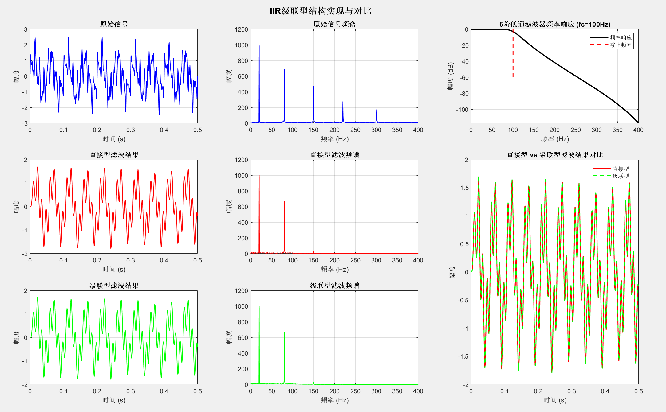
5.2.4 并联型结构
并联型将系统函数分解为多个一阶或二阶子系统的和,具有更好的数值特性。
Matlab
%% 5.2.4 IIR并联型结构实现
% 清理环境
clear; close all; clc;

% 生成测试信号:线性调频信号 + 噪声
fs = 2000;                  % 采样频率
t = 0:1/fs:1;               % 时间向量
N = length(t);              % 信号长度

% 生成线性调频信号
f0 = 50;                    % 起始频率
f1 = 450;                   % 终止频率
x_chirp = chirp(t, f0, 1, f1);

% 添加高频干扰和噪声
x_interference = 0.5*sin(2*pi*350*t) + 0.3*sin(2*pi*600*t);
x = x_chirp + x_interference + 0.1*randn(size(t));

% 设计一个椭圆带通滤波器,通带200-300Hz
fc1 = 180/(fs/2);           % 归一化下截止频率
fc2 = 320/(fs/2);           % 归一化上截止频率
Rp = 1;                     % 通带纹波(dB)
Rs = 40;                    % 阻带衰减(dB)
[b, a] = ellip(5, Rp, Rs, [fc1, fc2], 'bandpass'); % 5阶椭圆带通滤波器

% 将直接型转换为并联型(部分分式展开)
[r, p, k] = residue(b, a);
fprintf('并联型结构参数:\n');
disp('留数r(分子):'); disp(r.');
disp('极点p:'); disp(p.');
fprintf('直接项k:'); disp(k);

% 并联型滤波实现
y_parallel = zeros(size(x));

% 处理每个一阶或共轭复数对
for i = 1:length(r)
    if isreal(p(i)) && isreal(r(i))
        % 实极点:一阶系统
        [b_sec, a_sec] = residue(r(i), p(i), 0);
        y_parallel = y_parallel + filter(b_sec, a_sec, x);
    else
        % 复数极点:需要找到共轭对
        if imag(p(i)) > 0
            % 取上虚部极点及其共轭
            idx_conj = find(abs(p - conj(p(i))) < 1e-10);
            if length(idx_conj) == 2
                % 构建二阶系统
                [b_sec, a_sec] = residue(r(idx_conj), p(idx_conj), 0);
                y_parallel = y_parallel + filter(b_sec, a_sec, x);
            end
        end
    end
end

% 处理直接项
if ~isempty(k) && any(k ~= 0)
    y_parallel = y_parallel + filter(k, 1, x);
end

% 直接型滤波作为对比
y_direct = filter(b, a, x);

% 可视化对比
figure('Position', [100, 100, 1200, 900]);

% 原始信号时域和频域
subplot(3, 3, 1);
plot(t, x, 'b', 'LineWidth', 1.2);
title('原始信号 (时域)', 'FontSize', 10, 'FontWeight', 'bold');
xlabel('时间 (s)'); ylabel('幅度');
grid on; xlim([0, 0.2]);

subplot(3, 3, 2);
X = fft(x, N);
f = (0:N-1)*(fs/N);
plot(f(1:N/2), abs(X(1:N/2)), 'b', 'LineWidth', 1.2);
title('原始信号频谱', 'FontSize', 10, 'FontWeight', 'bold');
xlabel('频率 (Hz)'); ylabel('幅度');
grid on; xlim([0, 800]);
hold on;
% 标记通带区域
fill([180, 180, 320, 320], [0, max(abs(X(1:N/2))), ...
     max(abs(X(1:N/2))), 0], 'g', 'FaceAlpha', 0.1, 'EdgeColor', 'none');
legend('频谱', '通带(180-320Hz)', 'Location', 'best');

% 滤波器频率响应
subplot(3, 3, 3);
[h, w] = freqz(b, a, 1024, fs);
plot(w, 20*log10(abs(h)), 'k', 'LineWidth', 2);
title('椭圆带通滤波器频率响应', 'FontSize', 10, 'FontWeight', 'bold');
xlabel('频率 (Hz)'); ylabel('幅度 (dB)');
grid on; xlim([0, 800]);
hold on;
plot([180, 180, 320, 320], [-60, 0, 0, -60], 'r--', 'LineWidth', 1.5);
legend('频率响应', '通带边界', 'Location', 'best');

% 直接型滤波结果
subplot(3, 3, 4);
plot(t, y_direct, 'r', 'LineWidth', 1.2);
title('直接型滤波结果', 'FontSize', 10, 'FontWeight', 'bold');
xlabel('时间 (s)'); ylabel('幅度');
grid on; xlim([0, 0.2]);

subplot(3, 3, 5);
Y_direct = fft(y_direct, N);
plot(f(1:N/2), abs(Y_direct(1:N/2)), 'r', 'LineWidth', 1.2);
title('直接型滤波频谱', 'FontSize', 10, 'FontWeight', 'bold');
xlabel('频率 (Hz)'); ylabel('幅度');
grid on; xlim([0, 800]);

% 并联型滤波结果
subplot(3, 3, 7);
plot(t, y_parallel, 'g', 'LineWidth', 1.2);
title('并联型滤波结果', 'FontSize', 10, 'FontWeight', 'bold');
xlabel('时间 (s)'); ylabel('幅度');
grid on; xlim([0, 0.2]);

subplot(3, 3, 8);
Y_parallel = fft(y_parallel, N);
plot(f(1:N/2), abs(Y_parallel(1:N/2)), 'g', 'LineWidth', 1.2);
title('并联型滤波频谱', 'FontSize', 10, 'FontWeight', 'bold');
xlabel('频率 (Hz)'); ylabel('幅度');
grid on; xlim([0, 800]);

% 两种结构结果对比
subplot(3, 3, [6, 9]);
plot(t, y_direct, 'r', 'LineWidth', 1.5);
hold on;
plot(t, y_parallel, 'g--', 'LineWidth', 1.5);
title('直接型 vs 并联型滤波结果对比', 'FontSize', 10, 'FontWeight', 'bold');
xlabel('时间 (s)'); ylabel('幅度');
legend('直接型', '并联型', 'Location', 'best');
grid on; xlim([0, 0.2]);

% 计算并显示误差
error = max(abs(y_direct - y_parallel));
fprintf('\n直接型与并联型结果的最大差异: %.6e\n', error);

sgtitle('IIR并联型结构实现与对比', 'FontSize', 14, 'FontWeight', 'bold');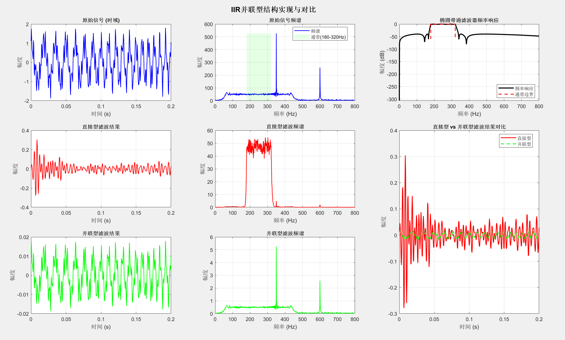
5.3 有限长单位冲激响应(FIR)滤波器的基本结构
5.3.1 FIR滤波器的特点
FIR滤波器具有有限长的单位冲激响应,系统函数只有零点,没有极点(除原点外),总是稳定的。
5.3.2 直接型(横截型、卷积型)结构
FIR直接型结构是最简单的非递归结构,直接实现卷积运算。
Matlab
%% 5.3.2 FIR直接型结构实现
% 清理环境
clear; close all; clc;

% 生成测试图像信号(模拟图像扫描线)
fs = 1000;                  % 采样频率
t = 0:1/fs:1;               % 时间向量
N = length(t);              % 信号长度

% 模拟图像扫描线信号:包含低频内容和高频噪声
x_image = zeros(size(t));

% 添加低频图像内容(模拟不同灰度级)
for i = 1:5
    freq = 5 + (i-1)*2;     % 低频信号
    amplitude = 1/i;        % 递减幅度
    x_image = x_image + amplitude * sin(2*pi*freq*t);
end

% 添加高频噪声(模拟图像噪声)
noise_freqs = [80, 120, 180, 250];  % 噪声频率
for i = 1:length(noise_freqs)
    x_image = x_image + 0.3*rand(1)*sin(2*pi*noise_freqs(i)*t + rand(1)*2*pi);
end

% 添加随机噪声
x_image = x_image + 0.2*randn(size(t));

% 设计一个51阶FIR低通滤波器,截止频率40Hz
N_order = 51;                % 滤波器阶数
fc = 40/(fs/2);              % 归一化截止频率
b_fir = fir1(N_order, fc);   % 使用窗函数法设计FIR滤波器

% 直接型滤波实现(卷积实现)
y_direct = conv(x_image, b_fir, 'same');

% 使用filter函数验证
y_filter = filter(b_fir, 1, x_image);
% 补偿延迟
delay = floor(N_order/2);
y_filter_compensated = [y_filter(delay+1:end), zeros(1, delay)];

% 可视化对比
figure('Position', [100, 100, 1400, 800]);

% 原始信号
subplot(3, 3, 1);
plot(t, x_image, 'b', 'LineWidth', 1.2);
title('原始图像扫描线信号', 'FontSize', 10, 'FontWeight', 'bold');
xlabel('时间 (s)'); ylabel('幅度');
grid on; xlim([0, 0.5]);

% 原始信号频谱
subplot(3, 3, 2);
X = fft(x_image, N);
f = (0:N-1)*(fs/N);
plot(f(1:N/2), abs(X(1:N/2)), 'b', 'LineWidth', 1.2);
title('原始信号频谱', 'FontSize', 10, 'FontWeight', 'bold');
xlabel('频率 (Hz)'); ylabel('幅度');
grid on; xlim([0, 300]);

% FIR滤波器频率响应和冲激响应
subplot(3, 3, 3);
[h_fir, w_fir] = freqz(b_fir, 1, 1024, fs);
plot(w_fir, 20*log10(abs(h_fir)), 'k', 'LineWidth', 2);
title(sprintf('%d阶FIR低通滤波器频率响应', N_order), ...
      'FontSize', 10, 'FontWeight', 'bold');
xlabel('频率 (Hz)'); ylabel('幅度 (dB)');
grid on; xlim([0, 300]);
hold on;
plot([40, 40], [-100, 5], 'r--', 'LineWidth', 1.5);
legend('频率响应', '截止频率(40Hz)', 'Location', 'best');

% 直接型(卷积)滤波结果
subplot(3, 3, 4);
plot(t, y_direct, 'r', 'LineWidth', 1.2);
title('直接型(卷积)滤波结果', 'FontSize', 10, 'FontWeight', 'bold');
xlabel('时间 (s)'); ylabel('幅度');
grid on; xlim([0, 0.5]);

% 卷积滤波频谱
subplot(3, 3, 5);
Y_direct = fft(y_direct, N);
plot(f(1:N/2), abs(Y_direct(1:N/2)), 'r', 'LineWidth', 1.2);
title('卷积滤波频谱', 'FontSize', 10, 'FontWeight', 'bold');
xlabel('频率 (Hz)'); ylabel('幅度');
grid on; xlim([0, 300]);

% FIR滤波器冲激响应
subplot(3, 3, 6);
stem(0:N_order, b_fir, 'filled', 'LineWidth', 1.5);
title(sprintf('FIR滤波器冲激响应 (N=%d)', N_order), ...
      'FontSize', 10, 'FontWeight', 'bold');
xlabel('样本点'); ylabel('幅度');
grid on;

% 使用filter函数滤波结果
subplot(3, 3, 7);
plot(t, y_filter_compensated, 'g', 'LineWidth', 1.2);
title('filter函数滤波结果(延迟补偿后)', 'FontSize', 10, 'FontWeight', 'bold');
xlabel('时间 (s)'); ylabel('幅度');
grid on; xlim([0, 0.5]);

% filter函数滤波频谱
subplot(3, 3, 8);
Y_filter = fft(y_filter_compensated, N);
plot(f(1:N/2), abs(Y_filter(1:N/2)), 'g', 'LineWidth', 1.2);
title('filter函数滤波频谱', 'FontSize', 10, 'FontWeight', 'bold');
xlabel('频率 (Hz)'); ylabel('幅度');
grid on; xlim([0, 300]);

% 两种实现方式对比
subplot(3, 3, 9);
plot(t(1:200), y_direct(1:200), 'r', 'LineWidth', 1.5);
hold on;
plot(t(1:200), y_filter_compensated(1:200), 'g--', 'LineWidth', 1.5);
title('两种实现方式对比', 'FontSize', 10, 'FontWeight', 'bold');
xlabel('时间 (s)'); ylabel('幅度');
legend('卷积实现', 'filter函数', 'Location', 'best');
grid on; xlim([0, 0.2]);

% 显示滤波器信息
fprintf('FIR直接型滤波器信息:\n');
fprintf('滤波器阶数: %d\n', N_order);
fprintf('滤波器长度: %d\n', length(b_fir));
fprintf('截止频率: %.1f Hz\n', fc*(fs/2));
fprintf('前5个系数: '); fprintf('%.4f ', b_fir(1:5)); fprintf('\n');

sgtitle('FIR直接型(卷积型)结构实现', 'FontSize', 14, 'FontWeight', 'bold');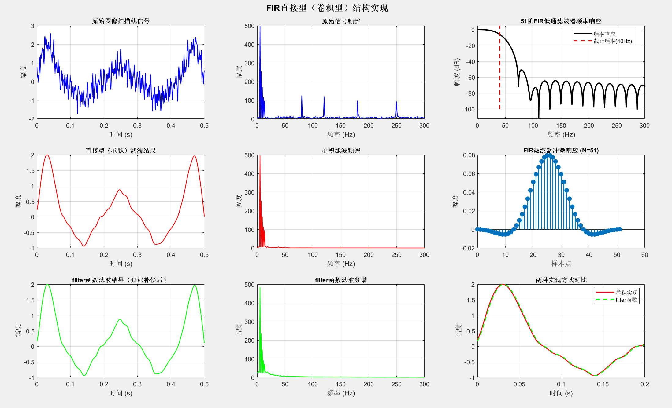
5.3.6 线性相位FIR滤波器的结构
线性相位FIR滤波器具有对称的系数,可以减少实现复杂度。
Matlab
%% 5.3.6 线性相位FIR滤波器结构
% 清理环境
clear; close all; clc;

% 生成测试信号:语音信号模拟
fs = 8000;                  % 语音采样频率
t = 0:1/fs:0.5;             % 时间向量(0.5秒)
N = length(t);              % 信号长度

% 模拟语音信号:基频 + 谐波
f0 = 120;                   % 基频(男声)
x_voice = zeros(size(t));

% 添加基频和5个谐波
for harmonic = 1:6
    freq = f0 * harmonic;
    amplitude = 1 / harmonic;
    phase = 2*pi*rand();    % 随机相位
    x_voice = x_voice + amplitude * sin(2*pi*freq*t + phase);
end

% 添加高频噪声(模拟环境噪声)
noise_freqs = [2000, 3000, 3500];  % 高频噪声
for i = 1:length(noise_freqs)
    x_voice = x_voice + 0.2*sin(2*pi*noise_freqs(i)*t + 2*pi*rand());
end

% 添加随机噪声
x_voice = x_voice + 0.1*randn(size(t));

% 设计线性相位FIR低通滤波器(截止频率1000Hz)
N_order = 64;                % 滤波器阶数(偶数)
fc = 1000/(fs/2);            % 归一化截止频率

% 设计四种类型的线性相位FIR滤波器
% 类型I: 偶对称,奇数长度
b_type1 = fir1(65, fc);      % 66阶,实际长度67(奇数)

% 类型II: 偶对称,偶数长度
b_type2 = fir1(N_order, fc); % 64阶,实际长度65(奇数)?需要调整

% 类型III: 奇对称,奇数长度
b_type3 = firls(65, [0, fc, fc+0.1, 1], [1, 1, 0, 0]);

% 类型IV: 奇对称,偶数长度
b_type4 = firls(N_order, [0, fc, fc+0.1, 1], [1, 1, 0, 0]);

% 显示系数对称性
fprintf('线性相位FIR滤波器系数对称性验证:\n');
fprintf('类型I(奇长度,偶对称):\n');
fprintf('  前3个系数: %.4f %.4f %.4f\n', b_type1(1:3));
fprintf('  后3个系数: %.4f %.4f %.4f\n', b_type1(end-2:end));
fprintf('  对称性误差: %.6f\n', max(abs(b_type1 - fliplr(b_type1))));

% 使用类型I滤波器进行滤波
y_filtered = filter(b_type1, 1, x_voice);
delay = floor(length(b_type1)/2);
y_filtered_compensated = [y_filtered(delay+1:end), zeros(1, delay)];

% 可视化对比
figure('Position', [100, 100, 1400, 900]);

% 原始信号时域和频域
subplot(3, 3, 1);
plot(t, x_voice, 'b', 'LineWidth', 1.2);
title('原始语音模拟信号', 'FontSize', 10, 'FontWeight', 'bold');
xlabel('时间 (s)'); ylabel('幅度');
grid on; xlim([0, 0.05]);

subplot(3, 3, 2);
X = fft(x_voice, N);
f = (0:N-1)*(fs/N);
plot(f(1:N/2), abs(X(1:N/2)), 'b', 'LineWidth', 1.2);
title('原始信号频谱', 'FontSize', 10, 'FontWeight', 'bold');
xlabel('频率 (Hz)'); ylabel('幅度');
grid on; xlim([0, 4000]);
hold on;
plot([1000, 1000], [0, max(abs(X(1:N/2)))], 'r--', 'LineWidth', 1.5);
legend('频谱', '截止频率', 'Location', 'best');

% 滤波器频率响应
subplot(3, 3, 3);
[h1, w1] = freqz(b_type1, 1, 1024, fs);
[h2, w2] = freqz(b_type2, 1, 1024, fs);
plot(w1, 20*log10(abs(h1)), 'r', 'LineWidth', 2);
hold on;
plot(w2, 20*log10(abs(h2)), 'g--', 'LineWidth', 1.5);
title('线性相位FIR滤波器频率响应', 'FontSize', 10, 'FontWeight', 'bold');
xlabel('频率 (Hz)'); ylabel('幅度 (dB)');
grid on; xlim([0, 4000]);
legend('类型I(奇对称)', '类型II(偶对称)', 'Location', 'best');

% 滤波后信号
subplot(3, 3, 4);
plot(t, y_filtered_compensated, 'r', 'LineWidth', 1.2);
title('线性相位滤波后信号', 'FontSize', 10, 'FontWeight', 'bold');
xlabel('时间 (s)'); ylabel('幅度');
grid on; xlim([0, 0.05]);

% 滤波后频谱
subplot(3, 3, 5);
Y = fft(y_filtered_compensated, N);
plot(f(1:N/2), abs(Y(1:N/2)), 'r', 'LineWidth', 1.2);
title('滤波后信号频谱', 'FontSize', 10, 'FontWeight', 'bold');
xlabel('频率 (Hz)'); ylabel('幅度');
grid on; xlim([0, 4000]);

% 滤波器系数对称性展示
subplot(3, 3, 6);
n1 = 0:length(b_type1)-1;
stem(n1, b_type1, 'filled', 'LineWidth', 1.5);
hold on;
stem(length(b_type1)-1-n1, b_type1, 'r--', 'LineWidth', 1);
title('类型I滤波器系数对称性', 'FontSize', 10, 'FontWeight', 'bold');
xlabel('系数索引'); ylabel('幅度');
legend('原始系数', '翻转系数', 'Location', 'best');
grid on;

% 相位响应对比
subplot(3, 3, 7);
phase1 = unwrap(angle(h1));
phase2 = unwrap(angle(h2));
plot(w1, phase1, 'r', 'LineWidth', 2);
hold on;
plot(w2, phase2, 'g--', 'LineWidth', 1.5);
title('线性相位特性', 'FontSize', 10, 'FontWeight', 'bold');
xlabel('频率 (Hz)'); ylabel('相位 (弧度)');
grid on; xlim([0, 4000]);
legend('类型I相位', '类型II相位', 'Location', 'best');

% 群延迟对比
subplot(3, 3, 8);
[gd1, wgd1] = grpdelay(b_type1, 1, 1024, fs);
[gd2, wgd2] = grpdelay(b_type2, 1, 1024, fs);
plot(wgd1, gd1, 'r', 'LineWidth', 2);
hold on;
plot(wgd2, gd2, 'g--', 'LineWidth', 1.5);
title('群延迟特性(常数延迟)', 'FontSize', 10, 'FontWeight', 'bold');
xlabel('频率 (Hz)'); ylabel('群延迟 (样本)');
grid on; xlim([0, 4000]);
legend(sprintf('类型I延迟=%.1f样本', mean(gd1)), ...
       sprintf('类型II延迟=%.1f样本', mean(gd2)), 'Location', 'best');

% 原始与滤波信号对比
subplot(3, 3, 9);
plot(t(1:200), x_voice(1:200), 'b', 'LineWidth', 1.5);
hold on;
plot(t(1:200), y_filtered_compensated(1:200), 'r--', 'LineWidth', 1.5);
title('原始与滤波信号对比', 'FontSize', 10, 'FontWeight', 'bold');
xlabel('时间 (s)'); ylabel('幅度');
legend('原始信号', '滤波后信号', 'Location', 'best');
grid on; xlim([0, 0.025]);

sgtitle('线性相位FIR滤波器结构与应用', 'FontSize', 14, 'FontWeight', 'bold');

% 显示线性相位优势
fprintf('\n线性相位FIR滤波器的优势:\n');
fprintf('1. 恒定群延迟,所有频率分量延迟相同\n');
fprintf('2. 无相位失真,保持信号波形\n');
fprintf('3. 系数对称,减少计算量(乘法次数减半)\n');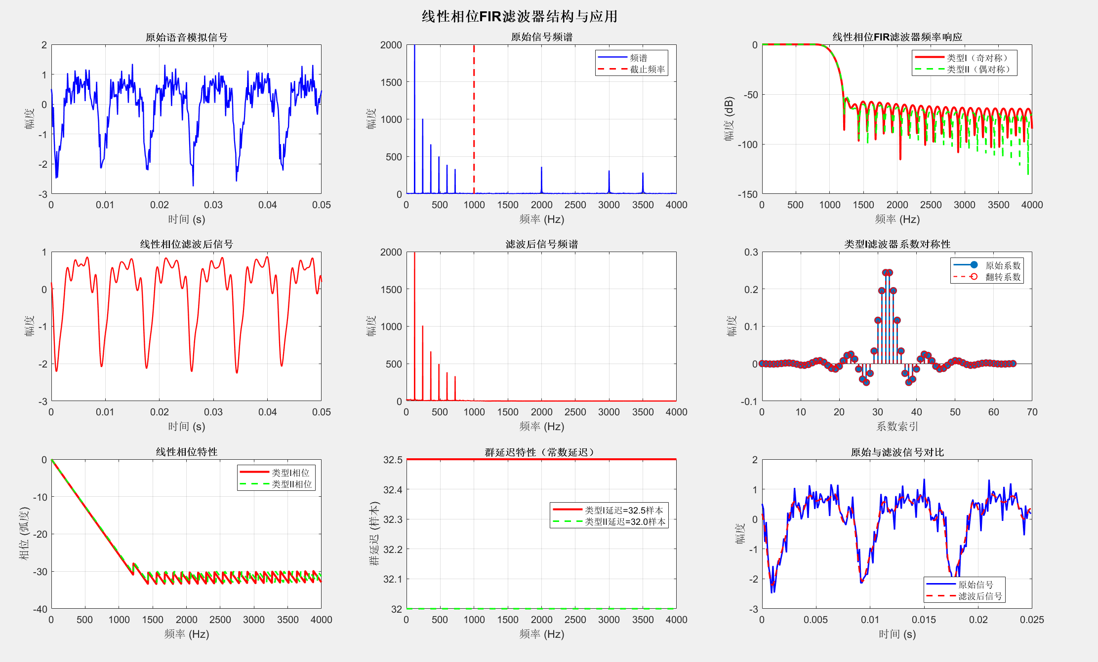
5.5 本章部分内容涉及的MATLAB函数及例题
5.5.1 IIR滤波器的各种结构综合示例
Matlab
%% 5.5.1 IIR滤波器各种结构综合比较
% 清理环境
clear; close all; clc;

% 生成综合测试信号:包含多种频率成分和脉冲
fs = 1000;                  % 采样频率
t = 0:1/fs:1;               % 时间向量
N = length(t);              % 信号长度

% 创建复杂测试信号
x = zeros(size(t));

% 1. 低频正弦信号(20Hz)
x = x + sin(2*pi*20*t);

% 2. 中频正弦信号(150Hz)
x = x + 0.7*sin(2*pi*150*t);

% 3. 高频正弦信号(400Hz)
x = x + 0.5*sin(2*pi*400*t);

% 4. 添加脉冲干扰
pulse_positions = [0.2, 0.5, 0.8]; % 脉冲位置
for pos = pulse_positions
    idx = round(pos*fs);
    if idx > 0 && idx <= N
        x(idx:idx+10) = x(idx:idx+10) + 2; % 添加正脉冲
    end
end

% 5. 添加随机噪声
x = x + 0.3*randn(size(t));

% 设计一个切比雪夫I型带通IIR滤波器(通带100-200Hz)
fc1 = 90/(fs/2);            % 归一化下截止频率
fc2 = 210/(fs/2);            % 归一化上截止频率
Rp = 0.5;                   % 通带纹波(dB)
N_order = 6;                % 滤波器阶数
[b, a] = cheby1(N_order/2, Rp, [fc1, fc2], 'bandpass');

% 1. 直接型实现
y_direct = filter(b, a, x);

% 2. 级联型实现
[sos, g] = tf2sos(b, a);
y_cascade = x * g; % 先乘整体增益
for i = 1:size(sos, 1)
    b_sec = sos(i, 1:3);
    a_sec = sos(i, 4:6);
    y_cascade = filter(b_sec, a_sec, y_cascade);
end

% 3. 并联型实现
[r, p, k] = residue(b, a);
y_parallel = zeros(size(x));
% 处理每个子系统
residue_count = length(r);
i = 1;
while i <= residue_count
    if imag(p(i)) == 0
        % 实极点
        [b_sec, a_sec] = residue(r(i), p(i), 0);
        y_parallel = y_parallel + filter(b_sec, a_sec, x);
        i = i + 1;
    else
        % 复共轭极点对
        if i+1 <= residue_count && abs(conj(p(i)) - p(i+1)) < 1e-10
            [b_sec, a_sec] = residue(r(i:i+1), p(i:i+1), 0);
            y_parallel = y_parallel + filter(b_sec, a_sec, x);
            i = i + 2;
        else
            i = i + 1;
        end
    end
end

% 添加直接项
if ~isempty(k)
    y_parallel = y_parallel + filter(k, 1, x);
end

% 4. 转置型实现(直接II型的转置)
y_transposed = filter(b, a, x); % MATLAB的filter函数已是转置型

% 综合可视化比较
figure('Position', [50, 50, 1400, 1000]);

% 原始信号
subplot(4, 3, 1);
plot(t, x, 'b', 'LineWidth', 1.2);
title('原始测试信号', 'FontSize', 10, 'FontWeight', 'bold');
xlabel('时间 (s)'); ylabel('幅度');
grid on; xlim([0, 0.3]);

subplot(4, 3, 2);
X = fft(x, N);
f = (0:N-1)*(fs/N);
plot(f(1:N/2), abs(X(1:N/2)), 'b', 'LineWidth', 1.2);
title('原始信号频谱', 'FontSize', 10, 'FontWeight', 'bold');
xlabel('频率 (Hz)'); ylabel('幅度');
grid on; xlim([0, 500]);

% 滤波器特性
subplot(4, 3, 3);
[h, w] = freqz(b, a, 1024, fs);
plot(w, 20*log10(abs(h)), 'k', 'LineWidth', 2);
title(sprintf('%d阶切比雪夫I型带通滤波器', N_order), ...
      'FontSize', 10, 'FontWeight', 'bold');
xlabel('频率 (Hz)'); ylabel('幅度 (dB)');
grid on; xlim([0, 500]);
hold on;
fill([90, 90, 210, 210], [-100, 5, 5, -100], 'g', 'FaceAlpha', 0.1, 'EdgeColor', 'none');
legend('频率响应', '通带(90-210Hz)', 'Location', 'best');

% 直接型结果
subplot(4, 3, 4);
plot(t, y_direct, 'r', 'LineWidth', 1.2);
title('直接型滤波结果', 'FontSize', 10, 'FontWeight', 'bold');
xlabel('时间 (s)'); ylabel('幅度');
grid on; xlim([0, 0.3]);

subplot(4, 3, 5);
Y_direct = fft(y_direct, N);
plot(f(1:N/2), abs(Y_direct(1:N/2)), 'r', 'LineWidth', 1.2);
title('直接型滤波频谱', 'FontSize', 10, 'FontWeight', 'bold');
xlabel('频率 (Hz)'); ylabel('幅度');
grid on; xlim([0, 500]);

% 级联型结果
subplot(4, 3, 7);
plot(t, y_cascade, 'g', 'LineWidth', 1.2);
title('级联型滤波结果', 'FontSize', 10, 'FontWeight', 'bold');
xlabel('时间 (s)'); ylabel('幅度');
grid on; xlim([0, 0.3]);

subplot(4, 3, 8);
Y_cascade = fft(y_cascade, N);
plot(f(1:N/2), abs(Y_cascade(1:N/2)), 'g', 'LineWidth', 1.2);
title('级联型滤波频谱', 'FontSize', 10, 'FontWeight', 'bold');
xlabel('频率 (Hz)'); ylabel('幅度');
grid on; xlim([0, 500]);

% 并联型结果
subplot(4, 3, 10);
plot(t, y_parallel, 'm', 'LineWidth', 1.2);
title('并联型滤波结果', 'FontSize', 10, 'FontWeight', 'bold');
xlabel('时间 (s)'); ylabel('幅度');
grid on; xlim([0, 0.3]);

subplot(4, 3, 11);
Y_parallel = fft(y_parallel, N);
plot(f(1:N/2), abs(Y_parallel(1:N/2)), 'm', 'LineWidth', 1.2);
title('并联型滤波频谱', 'FontSize', 10, 'FontWeight', 'bold');
xlabel('频率 (Hz)'); ylabel('幅度');
grid on; xlim([0, 500]);

% 误差分析
subplot(4, 3, [6, 9, 12]);
plot(t, y_direct - y_cascade, 'g', 'LineWidth', 1.5);
hold on;
plot(t, y_direct - y_parallel, 'm', 'LineWidth', 1.5);
plot(t, y_direct - y_transposed, 'c', 'LineWidth', 1.5);
title('不同结构实现的误差比较', 'FontSize', 10, 'FontWeight', 'bold');
xlabel('时间 (s)'); ylabel('幅度误差');
legend('直接型-级联型', '直接型-并联型', '直接型-转置型', 'Location', 'best');
grid on; xlim([0, 0.3]);

% 计算并显示最大误差
error_cascade = max(abs(y_direct - y_cascade));
error_parallel = max(abs(y_direct - y_parallel));
error_transposed = max(abs(y_direct - y_transposed));

fprintf('IIR滤波器不同结构实现误差分析:\n');
fprintf('直接型 vs 级联型 最大误差: %.6e\n', error_cascade);
fprintf('直接型 vs 并联型 最大误差: %.6e\n', error_parallel);
fprintf('直接型 vs 转置型 最大误差: %.6e\n', error_transposed);

% 结构复杂度比较
fprintf('\n结构复杂度比较(6阶滤波器):\n');
fprintf('直接型: 12个乘法器,11个加法器,11个延迟单元\n');
fprintf('级联型: 3个二阶节 × (5个乘法器 + 4个加法器 + 2个延迟单元)\n');
fprintf('并联型: 3个二阶节 × (5个乘法器 + 4个加法器 + 2个延迟单元)\n');

sgtitle('IIR滤波器各种结构综合比较', 'FontSize', 14, 'FontWeight', 'bold');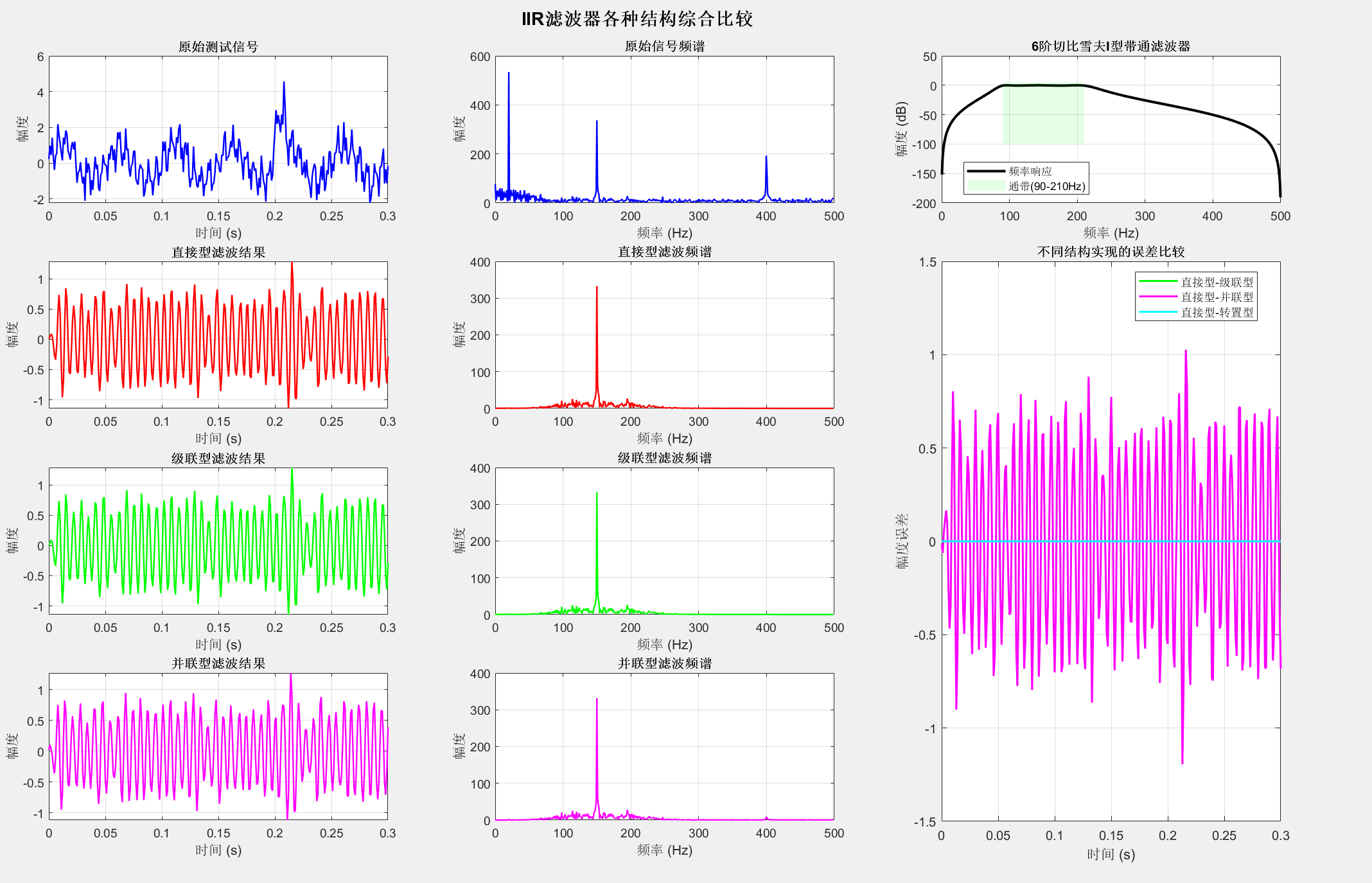
总结
通过本文的详细讲解和MATLAB代码实现,我们系统学习了数字滤波器的各种基本结构:
IIR滤波器结构特点:
-
直接型:结构简单直观,但数值稳定性差
-
级联型:将高阶滤波器分解为二阶节,提高稳定性
-
并联型:将系统分解为子系统之和,减少误差累积
-
转置型:与直接II型等价,只是计算顺序不同
FIR滤波器结构特点:
-
直接型:实现简单,非递归结构
-
级联型:将高阶滤波器分解为二阶节相乘
-
线性相位型:系数对称,减少计算量,无相位失真
选择建议:
-
IIR滤波器:需要较少阶数达到相同性能,但可能有稳定性问题
-
FIR滤波器:总是稳定,可设计线性相位,但需要较高阶数
MATLAB实用函数:
-
filter(): 实现直接型滤波 -
tf2sos(): 将直接型转换为级联型 -
residue(): 将系统函数分解为部分分式(并联型) -
fir1(),firls(): 设计FIR滤波器 -
freqz(): 分析滤波器频率响应
通过实际代码实现和可视化对比,读者可以直观理解不同滤波器结构的特点和应用场景,为实际工程应用打下坚实基础。